This page was generated by nbsphinx from docs/notebooks/diagnostics/charged_particle_radiography_particle_tracing_wire_mesh.ipynb.
Interactive online version: .

Synthetic Charged Particle Radiographs with a Wire Mesh

In charged particle radiography experiments a wire mesh grid is often placed between the particle source and the object of interest, leaving a shadow of the grid in the particle fluence. The displacement of these shadow grid lines can then be used to quantitatively extract the line-integrated force experienced at each grid vertex.

The Tracker class includes a method (add_wire_mesh()) that can be used to create synthetic radiographs with a mesh in place. In this example notebook we will illustrate the options available for creating and placing the mesh(s), the demonstrate the use of a mesh grid in a practical example.

import warnings

import astropy.units as u
import matplotlib.pyplot as plt
import numpy as np

from plasmapy.diagnostics.charged_particle_radiography import (
    synthetic_radiography as cpr,
)
from plasmapy.plasma.grids import CartesianGrid

Creating and Placing a Wire Mesh

We will begin by creating an empty CartesianGrid object in which the electric and magnetic fields are zero. Particle tracing through this grid will allow us to image just the mesh once we add one in place.

empty_grid = CartesianGrid(-1 * u.mm, 1 * u.mm, num=50)

The charged particle radiography Tracker will warn us every time we use this grid that the fields are not specified (before assuming that they are zero). The following line will silence this warning.

warnings.simplefilter("ignore")

We’ll also define a fixed source and detector that we won’t change for the rest of the example.

source = (0 * u.mm, -10 * u.mm, 0 * u.mm)
detector = (0 * u.mm, 200 * u.mm, 0 * u.mm)

Finally, we’ll create an instance of Tracker.

sim = cpr.Tracker(empty_grid, source, detector, verbose=False)

Now it’s time to create the mesh. add_wire_mesh() takes four required parameters:

• location : A vector from the grid origin to the center of the mesh.

• extent : The size of the mesh. If two values are given the mesh is assumed to be rectangular (extent is the width, height), but if only one is provided the mesh is assumed to be circular (extent is the diameter).

• nwires : The number of wires in each direction. If only one value is given, it’s assumed to be the same for both directions.

• wire_diameter : The diameter of each wire.

add_wire_mesh() works by extrapolating the positions of the particles in the mesh plane (based on their initial velocities) and removing those particles that will hit the wires. When add_wire_mesh() is called, the description of the mesh is stored inside the Tracker object. Multiple meshes can be added. The particles are then removed when the run() method is called.

location = np.array([0, -2, 0]) * u.mm
extent = (1 * u.mm, 1 * u.mm)
nwires = (9, 12)
wire_diameter = 20 * u.um
sim.add_wire_mesh(location, extent, nwires, wire_diameter)

Now that the mesh has been created, we will run the particle tracing simulation and create a synthetic radiograph to visualize the result. We’ll wrap this in a function so we can use it again later.

def run_radiograph(sim, vmax=None):
    sim.create_particles(1e5, 15 * u.MeV, max_theta=8 * u.deg)
    sim.run(field_weighting="nearest neighbor")
    h, v, i = cpr.synthetic_radiograph(
        sim, size=np.array([[-1, 1], [-1, 1]]) * 1.8 * u.cm, bins=[200, 200]
    )

    if vmax is None:
        vmax = np.max(i)

    fig, ax = plt.subplots(figsize=(8, 8))
    ax.pcolormesh(h.to(u.mm).value, v.to(u.mm).value, i.T, cmap="Blues_r", vmax=vmax)
    ax.set_aspect("equal")
    ax.set_xlabel("X (mm)")
    ax.set_ylabel("Y (mm)")

run_radiograph(sim)

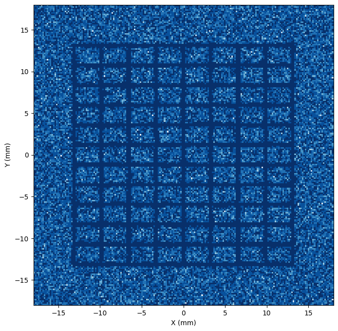
Notice that the distance from the source to the mesh is \(10 - 2 = 8\) mm, while the distance from the mesh to the detector is \(200 + 2 = 202\) mm. The magnification is therefore \(M = 1 + 202/8 = 26.25\), so the \(1\) mm wide mesh is \(26.25\) mm wide in the image.

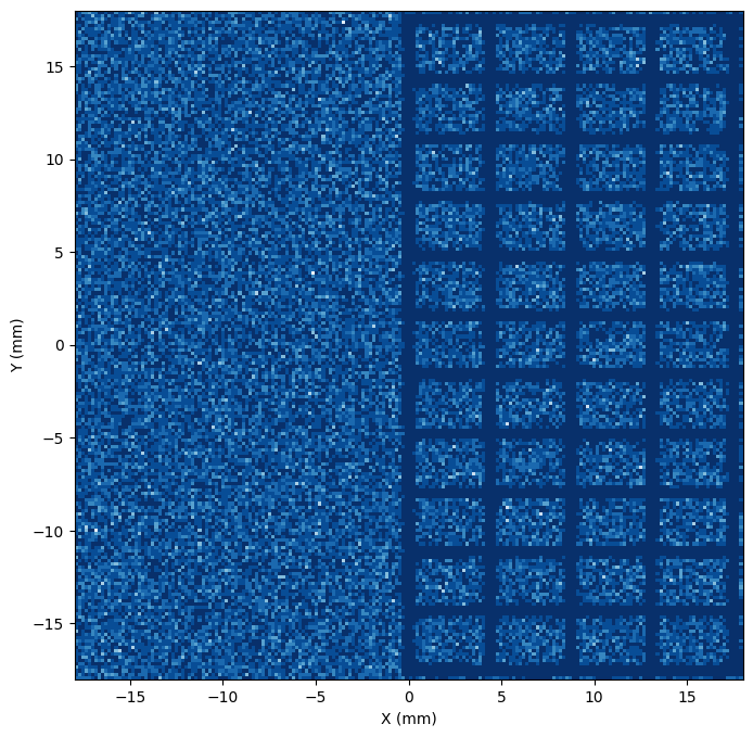
Changing the location keyword can change both the magnification and shift the mesh center.

sim = cpr.Tracker(empty_grid, source, detector, verbose=False)
sim.add_wire_mesh(np.array([0.5, -4, 0]) * u.mm, extent, nwires, wire_diameter)
run_radiograph(sim)

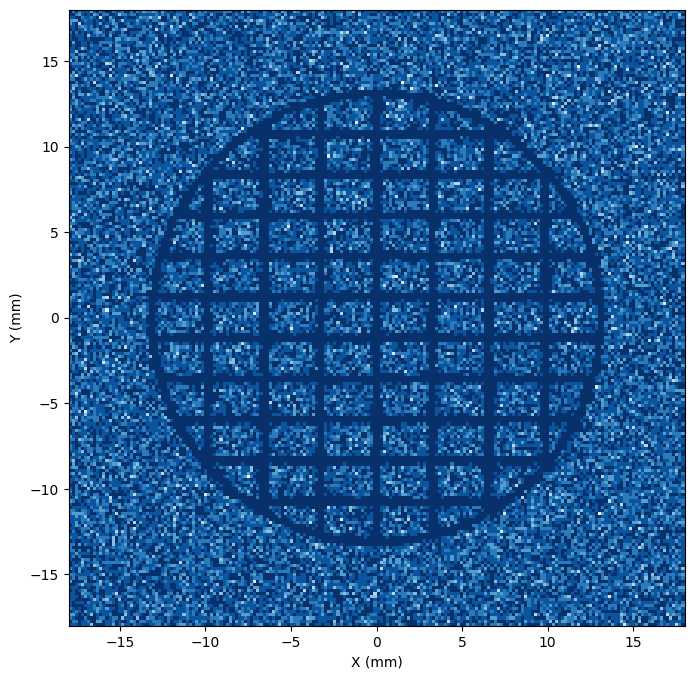
Setting the extent keyword to a single value will create a circular mesh (with a rectangular grid of wires).

sim = cpr.Tracker(empty_grid, source, detector, verbose=False)
sim.add_wire_mesh(location, (1 * u.mm), nwires, wire_diameter)
run_radiograph(sim)

add_wire_mesh() has two optional keywords that can be used to change the orientation of the mesh. The first, mesh_hdir is a unit vector that sets the horizontal direction of the mesh plane. This can be used to effectively rotate the mesh. For example the following example will rotate the mesh by \(45^\circ\) (note that these unit vector inputs are automatically normalized).

sim = cpr.Tracker(empty_grid, source, detector, verbose=False)
nremoved = sim.add_wire_mesh(
    location, extent, nwires, wire_diameter, mesh_hdir=np.array([0.5, 0, 0.5])
)
run_radiograph(sim)

The second keyword argument, mesh_vdir, overrides the unit vector that defines the vertical direction of the mesh plane. By default this vector is set to be mutually orthogonal to mesh_hdir and the detector plane normal so that the mesh is parallel to the detector plane. Changing this keyword (alone or in combination with mesh_hdir) can be used to create a tilted mesh.

sim = cpr.Tracker(empty_grid, source, detector, verbose=False)
nremoved = sim.add_wire_mesh(
    location, extent, nwires, wire_diameter, mesh_vdir=np.array([0, 0.7, 1])
)
run_radiograph(sim)

Using a Wire Mesh in an Example Radiograph

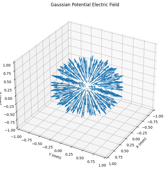
To illustrate the use of a mesh in an actual example, we’ll first create an example CartesianGrid object and fill it with the analytical electric field produced by a sphere of Gaussian potential.

# Create a Cartesian grid
L = 1 * u.mm
grid = CartesianGrid(-L, L, num=150)

# Create a spherical potential with a Gaussian radial distribution
radius = np.linalg.norm(grid.grid, axis=3)
arg = (radius / (L / 3)).to(u.dimensionless_unscaled)
potential = 2e5 * np.exp(-(arg**2)) * u.V

# Calculate E from the potential
Ex, Ey, Ez = np.gradient(potential, grid.dax0, grid.dax1, grid.dax2)
Ex = -np.where(radius < L / 2, Ex, 0)
Ey = -np.where(radius < L / 2, Ey, 0)
Ez = -np.where(radius < L / 2, Ez, 0)

# Add those quantities to the grid
grid.add_quantities(E_x=Ex, E_y=Ey, E_z=Ez, phi=potential)


# Plot the E-field
fig = plt.figure(figsize=(8, 8))
ax = fig.add_subplot(111, projection="3d")
ax.view_init(30, 30)

# skip some points to make the vector plot intelligible
s = tuple([slice(None, None, 10)] * 3)

ax.quiver(
    grid.pts0[s].to(u.mm).value,
    grid.pts1[s].to(u.mm).value,
    grid.pts2[s].to(u.mm).value,
    grid["E_x"][s],
    grid["E_y"][s],
    grid["E_z"][s],
    length=1e-6,
)

ax.set_xlabel("X (mm)")
ax.set_ylabel("Y (mm)")
ax.set_zlabel("Z (mm)")
ax.set_xlim(-1, 1)
ax.set_ylim(-1, 1)
ax.set_zlim(-1, 1)
ax.set_title("Gaussian Potential Electric Field");

Now we will create a mesh and run the particle tracing simulation

sim = cpr.Tracker(grid, source, detector, verbose=False)
sim.add_wire_mesh(location, extent, 11, wire_diameter)
sim.create_particles(3e5, 15 * u.MeV, max_theta=8 * u.deg)
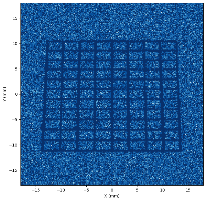
run_radiograph(sim, vmax=10)

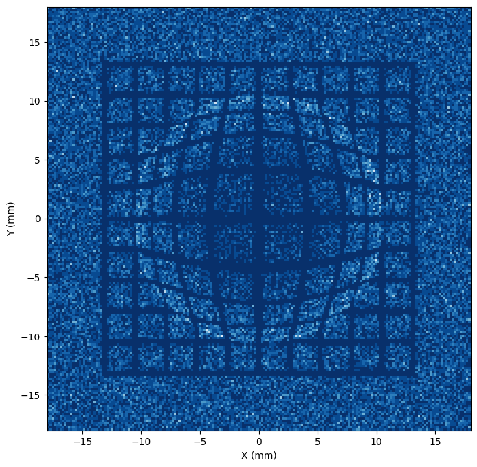
Notice how the vertices of the grid are displaced by the fields.