This page was generated by nbsphinx from docs/notebooks/formulary/thermal_bremsstrahlung.ipynb.
Interactive online version: .

Emission of Thermal Bremsstrahlung by a Maxwellian Plasma

The radiation.thermal_bremsstrahlung function calculates the bremsstrahlung spectrum emitted by the collision of electrons and ions in a thermal (Maxwellian) plasma. This function calculates this quantity in the Rayleigh-Jeans limit where \(\hbar\omega \ll k_B T_e\). In this regime, the power spectrum of the emitted radiation is

\begin{equation} \frac{dP}{d\omega} = \frac{8 \sqrt{2}}{3\sqrt{\pi}} \bigg ( \frac{e^2}{4 \pi \epsilon_0} \bigg )^3 \bigg ( m_e c^2 \bigg )^{-\frac{3}{2}} \bigg ( 1 - \frac{\omega_{pe}^2}{\omega^2} \bigg )^\frac{1}{2} \frac{Z_i^2 n_i n_e}{\sqrt{k_B T_e}} E_1(y) \end{equation}

where \(w_{pe}\) is the electron plasma frequency and \(E_1\) is the exponential integral

\begin{equation} E_1 (y) = - \int_{-y}^\infty \frac{e^{-t}}{t}dt \end{equation}

and y is the dimensionless argument

\begin{equation} y = \frac{1}{2} \frac{\omega^2 m_e}{k_{max}^2 k_B T_e} \end{equation}

where \(k_{max}\) is a maximum wavenumber arising from binary collisions approximated here as

\begin{equation} k_{max} = \frac{1}{\lambda_B} = \frac{\sqrt{m_e k_B T_e}}{\hbar} \end{equation}

where \(\lambda_B\) is the electron de Broglie wavelength. In some regimes other values for \(k_{max}\) may be appropriate, so its value may be set using a keyword. Bremsstrahlung emission is greatly reduced below the electron plasma frequency (where the plasma is opaque to EM radiation), so these expressions are only valid in the regime \(w < w_{pe}\).

%matplotlib inline

import astropy.constants as const
import astropy.units as u
import matplotlib.pyplot as plt
import numpy as np

from plasmapy.formulary.radiation import thermal_bremsstrahlung

Create an array of frequencies over which to calculate the bremsstrahlung spectrum and convert these frequencies to photon energies for the purpose of plotting the results. Set the plasma density, temperature, and ion species.

frequencies = np.arange(15, 16, 0.01)
frequencies = (10**frequencies) / u.s

energies = (frequencies * const.h.si).to(u.eV)

ne = 1e22 * u.cm**-3
Te = 1e2 * u.eV
ion = "C-12 4+"

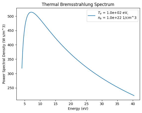
Calculate the spectrum, then plot it.

spectrum = thermal_bremsstrahlung(frequencies, ne, Te, ion=ion)

print(spectrum.unit)

lbl = f"$T_e$ = {Te.value:.1e} eV,\n" + f"$n_e$ = {ne.value:.1e} 1/cm^3"
plt.plot(energies, spectrum, label=lbl)
plt.title("Thermal Bremsstrahlung Spectrum")
plt.xlabel("Energy (eV)")
plt.ylabel("Power Spectral Density (W s/m^3)")
plt.legend()
plt.show()

kg / (m s2)

The power spectrum is the power per angular frequency per volume integrated over \(4\pi\) sr of solid angle, and therefore has units of watts / (rad/s) / m\(^3\) * \(4\pi\) rad = W s/m\(^3\).

spectrum = spectrum.to(u.W * u.s / u.m**3)
spectrum.unit

$\mathrm{\frac{W\,s}{m^{3}}}$

This means that, for a given volume and time period, the total energy emitted can be determined by integrating the power spectrum

t = 5 * u.ns
vol = 0.5 * u.cm**3
dw = 2 * np.pi * np.gradient(frequencies)  # Frequency step size
total_energy = (np.sum(spectrum * dw) * t * vol).to(u.J)
print(f"Total Energy: {total_energy.value:.2e} J")

Total Energy: 4.97e+04 J