This page was generated by
nbsphinx from
docs/notebooks/particles/ace.ipynb.
Interactive online version:
![]() .
.
Ionization states in an interplanetary coronal mass ejection
The ionization state distribution for an element refers to the fractions of that element at each ionic level. For example, the ionization state of helium in the solar wind might be 10% He\(^{0+}\), 70% He\(^{1+}\), and 20% He\(^{2+}\). This notebook introduces the data structures in plasmapy.particles for representing the ionization state of a plasma.
[1]:
import astropy.units as u
import matplotlib.pyplot as plt

from plasmapy.particles import IonizationState, IonizationStateCollection
The ionization state of a single element
Let’s create an IonizationState object for helium using the ionic fractions described above. We’ll specify the total number density of helium via the n_elem keyword argument.
[2]:
He_states = IonizationState("He-4", [0.1, 0.7, 0.2], n_elem=1e13 * u.m**-3)
The ionization state distribution is stored in the ionic_fractions attribute of IonizationState.
[3]:
array([0.1, 0.7, 0.2])
We can get the symbols for each ionic level in He_states too.
[4]:
['He-4 0+', 'He-4 1+', 'He-4 2+']
Because we provided the number density of the element as a whole, we can get back the number density of each ionic level.
[5]:
We can also get the electron number density required to balance the positive charges for ions of this element.
[6]:
[6]:
We can provide an IonizationState with a charge number as an index to get an IonicLevel object that contains most of these attributes, but for a single ionic level (like He\(^{1+}\)). This capability is useful if we wish to iterate over the ions of an element.
IonicLevel('He-4 0+', ionic_fraction=0.1)
IonicLevel('He-4 1+', ionic_fraction=0.7)
IonicLevel('He-4 2+', ionic_fraction=0.2)
We can get information about the average charge state via Z_mean, Z_most_abundant, and Z_rms.
[8]:
[8]:
np.float64(1.1)
[9]:
[1]
[10]:
[10]:
np.float64(1.224744871391589)
We can calculate the properties of the average ionic level.
[11]:
[11]:
CustomParticle(mass=6.645477039375987e-27 kg, charge=1.7623942974e-19 C)
We can use the summarize() method to get information about the ionization state.
[12]:
IonizationState instance for He-4 with Z_mean = 1.10
----------------------------------------------------------------
He-4  0+: 0.100    n_i = 1.00e+12 m**-3
He-4  1+: 0.700    n_i = 7.00e+12 m**-3
He-4  2+: 0.200    n_i = 2.00e+12 m**-3
----------------------------------------------------------------
n_elem = 1.00e+13 m**-3
n_e = 1.10e+13 m**-3
----------------------------------------------------------------
Ionization states of multiple elements
Now let’s look at some actual average hourly densities for ions of C, O, and Fe during an interplanetary coronal mass ejection (ICME) observed by the Advanced Composition Explorer (ACE) near 1 AU. The data were estimated from Figure 4 in Gilbert et al. (2012). This data set is noteworthy because there is information from very low charge states to very high charge states for several elements.
The electron ionization and radiative recombination rates for a given temperature are proportional to \(n_i n_e\), where \(n_i\) is the ion number density and \(n_e\) is the electron number density. Ionization and recombination are fast at high densities and slow at low densities. High density plasma can reach ionization equilibrium (when the recombination and ionization rates balance each other out) more quickly than low density plasma. Plasma undergoing rapid heating or cooling will be in non-equilibrium ionization because ionization and recombination can’t keep up with the temperature changes.
Quiescent plasma near the sun is typically close to ionization equilibrium because the density is high. As plasma moves away from the sun, the ionization and recombination rates drop rapidly because of the decreasing number density. The ionization states freeze out at several solar radii as the ionization and recombination time scales begin to exceed the time it takes for plasma to move from the sun to 1 AU.
The ionization states of the solar wind are powerful diagnostics of the thermodynamic history of solar wind and ICME plasma. The ionization states observed by ACE at 1 AU are essentially the same as at ∼\(5R_☉\).
[13]:
number_densities = {
    "C": [0, 5.7e-7, 4.3e-5, 3.6e-6, 2.35e-6, 1e-6, 1.29e-6] * u.cm**-3,
    "O": [0, 1.2e-7, 2.2e-4, 7.8e-6, 8.8e-7, 1e-6, 4e-6, 1.3e-6, 1.2e-7] * u.cm**-3,
    "Fe": [
        0,
        0,
        1.4e-8,
        1.1e-7,
        2.5e-7,
        2.2e-7,
        1.4e-7,
        1.2e-7,
        2.1e-7,
        2.1e-7,
        1.6e-7,
        8e-8,
        6.3e-8,
        4.2e-8,
        2.5e-8,
        2.3e-8,
        1.5e-8,
        3.1e-8,
        6.1e-9,
        2.3e-9,
        5.3e-10,
        2.3e-10,
        0,
        0,
        0,
        0,
        0,
    ]
    * u.cm**-3,
}
Let’s use this information as an input for IonizationStateCollection: a data structure for the ionization states of multiple elements.
[14]:
states = IonizationStateCollection(number_densities)
We can index this to get an IonizationState for one of the elements.
[15]:
states["C"]
[15]:
<IonizationState instance for C>
We can get the relative abundances of each of the elements.
[16]:
[16]:
{'C': 0.17942722921968796, 'O': 0.8146086249190311, 'Fe': 0.005964145861281176}
[17]:
[17]:
{'C': np.float64(-0.7461116493492604),
 'O': np.float64(-0.08905099599945356),
 'Fe': np.float64(-2.224451743828212)}
We can get the number densities as a dict (like what we provided) and the electron number density (assuming quasineutrality, but only for the elements contained in the data structure).
[18]:
[18]:
{'C': <Quantity [ 0.  ,  0.57, 43.  ,  3.6 ,  2.35,  1.  ,  1.29] 1 / m3>,
 'O': <Quantity [0.0e+00, 1.2e-01, 2.2e+02, 7.8e+00, 8.8e-01, 1.0e+00, 4.0e+00,
            1.3e+00, 1.2e-01] 1 / m3>,
 'Fe': <Quantity [0.0e+00, 0.0e+00, 1.4e-02, 1.1e-01, 2.5e-01, 2.2e-01, 1.4e-01,
            1.2e-01, 2.1e-01, 2.1e-01, 1.6e-01, 8.0e-02, 6.3e-02, 4.2e-02,
            2.5e-02, 2.3e-02, 1.5e-02, 3.1e-02, 6.1e-03, 2.3e-03, 5.3e-04,
            2.3e-04, 0.0e+00, 0.0e+00, 0.0e+00, 0.0e+00, 0.0e+00] 1 / m3>}
[19]:
[19]:
We can summarize this information too, but let’s specify the minimum ionic fraction to print.
[20]:
states.summarize(minimum_ionic_fraction=0.02)
IonizationStateCollection instance for: C, O, Fe
----------------------------------------------------------------
C  2+: 0.830    n_i = 4.30e+01 m**-3
C  3+: 0.069    n_i = 3.60e+00 m**-3
C  4+: 0.045    n_i = 2.35e+00 m**-3
C  6+: 0.025    n_i = 1.29e+00 m**-3
----------------------------------------------------------------
O  2+: 0.935    n_i = 2.20e+02 m**-3
O  3+: 0.033    n_i = 7.80e+00 m**-3
----------------------------------------------------------------
Fe  3+: 0.064    n_i = 1.10e-01 m**-3
Fe  4+: 0.145    n_i = 2.50e-01 m**-3
Fe  5+: 0.128    n_i = 2.20e-01 m**-3
Fe  6+: 0.081    n_i = 1.40e-01 m**-3
Fe  7+: 0.070    n_i = 1.20e-01 m**-3
Fe  8+: 0.122    n_i = 2.10e-01 m**-3
Fe  9+: 0.122    n_i = 2.10e-01 m**-3
Fe 10+: 0.093    n_i = 1.60e-01 m**-3
Fe 11+: 0.046    n_i = 8.00e-02 m**-3
Fe 12+: 0.037    n_i = 6.30e-02 m**-3
Fe 13+: 0.024    n_i = 4.20e-02 m**-3
----------------------------------------------------------------
n_e = 6.39e+02 m**-3
----------------------------------------------------------------
[21]:
fig, axes = plt.subplots(1, 3, figsize=(10, 3), tight_layout=True)

for state, ax in zip(states, axes, strict=False):
    ax.bar(state.charge_numbers, state.ionic_fractions)
    ax.set_title(f"Ionization state for {state.base_particle}")
    ax.set_xlabel("ionic level")
    ax.set_ylabel("log$_{10}$ of ionic fraction")
    ax.set_yscale("log")
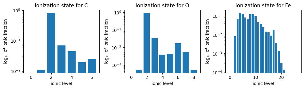
The wide range of average ionic levels for each element is strong evidence that the plasma observed by ACE originated from a wide range of temperatures. The lowest charge states are evidence of cool filament plasma while the high charge states are evidence of rapidly heated plasma.