This page was generated by nbsphinx from docs/notebooks/dispersion/stix_dispersion.ipynb.
Interactive online version: .

Stix Dispersion Solver

This notebook details the functionality of the stix() function. This is an analytical solution of equation 8 in Bellan 2012, the function is defined by Stix 1992 in §1.2 to be:

\[(S \sin^2(θ) + P \cos^2(θ)) \left ( \frac{ck}{ω} \right)^4 - [ RL \sin^2(θ) + PS (1 + \cos^2(θ)) ] \left ( \frac{ck}{ω} \right)^2 + PRL = 0\]

where,

\[\begin{split}\mathbf{B}_0 = B_0 \mathbf{\hat{z}} \cos θ = \frac{k_z}{k} \\ \mathbf{k} = k_{\rm x} \hat{x} + k_{\rm z} \hat{z}\end{split}\]

\[S = 1 - \sum_s \frac{ω^2_{p,s}}{ω^2 - ω^2_{c,s}}\hspace{2.5cm} P = 1 - \sum_s \frac{ω^2_{p,s}}{ω^2}\hspace{2.5cm} D = \sum_s \frac{ω_{c,s}}{ω} \frac{ω^2_{p,s}}{ω^2 - ω_{c,s}^2}\]

\[R = S + D \hspace{1cm} L = S - D\]

\(ω\) is the wave frequency, \(k\) is the wavenumber, \(θ\) is the wave propagation angle with respect to the background magnetic field \(\mathbf{B}_0\), \(s\) corresponds to plasma species, \(ω_{p,s}\) is the plasma frequency of species and \(ω_{c,s}\) is the gyrofrequency of species \(s\).

Note

The derivation of this dispersion relation assumed:

• zero temperature for all plasma species (\(T_s=0\))

• quasineutrality

• a uniform background magnetic field \(\mathbf{B_0} = B_0 \mathbf{\hat{z}}\)

• no D.C. electric field \(\mathbf{E_0}=0\)

• zero-order quantities for all plasma parameters (densities, electric-field, magnetic field, particle speeds, etc.) are constant in time and space

• first-order perturbations in plasma parameters vary like \(\sim e^{\left [ i (\textbf{k}\cdot\textbf{r} - \omega t)\right ]}\)

Due to the cold plasma assumption, this equation is valid for all \(ω\) and \(k\) given \(\frac{ω}{k_z} ≫ v_{Th}\) for all thermal speeds \(v_{Th}\) of all plasma species and \(k_x r_L ≪ 1\) for all gyroradii \(r_L\) of all plasma species. The relation predicts \(k → 0\) when any one of P, R or L vanish (cutoffs) and \(k → ∞\) for perpendicular propagation during wave resonance \(S → 0\).

Contents

1. Wave Normal to the Surface

2. Comparison with Bellan

import functools

import astropy.units as u
import matplotlib.pyplot as plt
import numpy as np
import scipy
from astropy.constants.si import c

from plasmapy.dispersion.analytical.stix_ import stix
from plasmapy.dispersion.analytical.two_fluid_ import two_fluid
from plasmapy.formulary import speeds
from plasmapy.particles import Particle

plt.rcParams["figure.figsize"] = [10.5, 0.56 * 10.5]

Wave Normal to the Surface

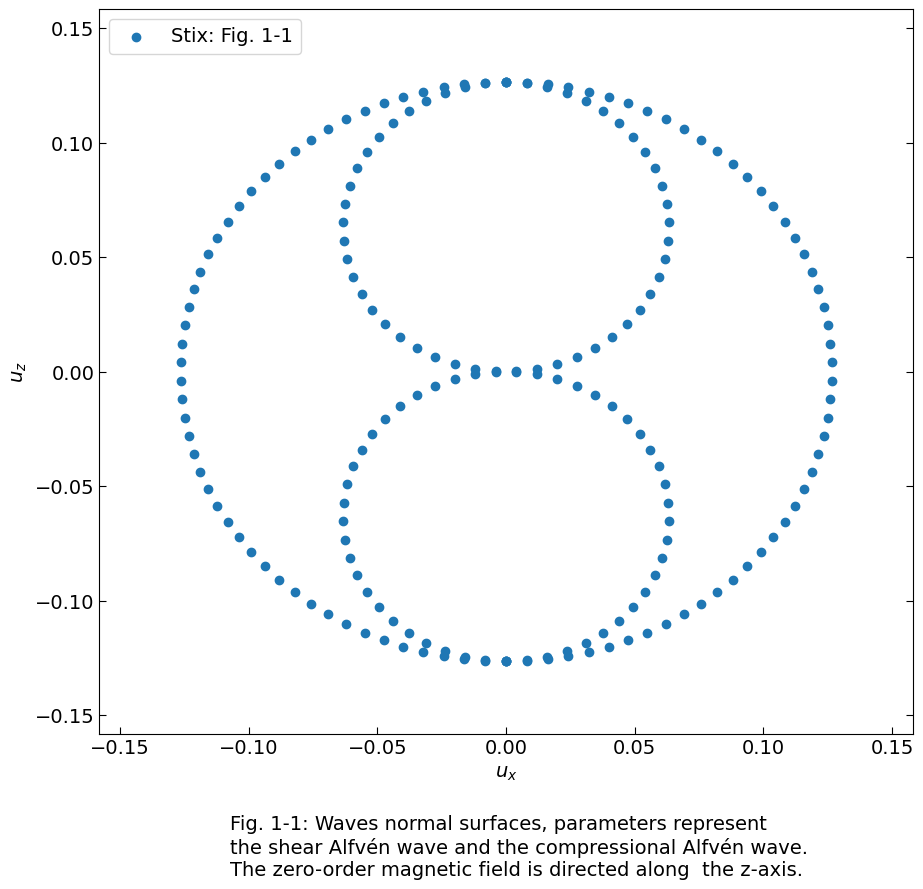
To calculate the normal surface waves propagating through a magnetized uniform cold plasma. The wave which is normal to the surface, is the locus of the phase velocity \(\textbf{v}_{phase} = \frac{ω}{k} \, \hat{k}\) where \(\hat{k} = \frac{\textbf{k}}{k}\). The equation for the wave normal surface can be derived via the prior equations, resulting in the form of

\[A u^4 + B u^2 + C = 0\]

where \(u = \frac{ω}{ck}\). To begin we define the required parameters to compute the wave numbers.

# define input parameters
inputs_1 = {
    "theta": np.linspace(0, np.pi, 50) * u.rad,
    "ions": Particle("p"),
    "n_i": 1e12 * u.cm**-3,
    "B": 0.43463483142776164 * u.T,
    "w": 41632.94534008216 * u.rad / u.s,
}

# define a meshgrid based on the number of theta values
omegas, thetas = np.meshgrid(
    inputs_1["w"].value, inputs_1["theta"].value, indexing="ij"
)
omegas = np.dstack((omegas,) * 4).squeeze()
thetas = np.dstack((thetas,) * 4).squeeze()

# compute k values
k = stix(**inputs_1)

The computed wavenumbers in units (rad/m) are returned in a dictionary (shape \(N × M × 4\)), with the keys representing \(θ\) and the values (instances of Astropy Quantity) being the wavenumbers. The first dimension maps to the \(w\) array, the second dimension maps to the \(θ\) array, and the third dimension maps to the four roots of the Stix polynomial.

• \(k[0]\) is the square root of the positive quadratic solution

• \(k[1] = -k[0]\)

• \(k[2]\) is the square root of the negative quadratic solution

• \(k[3] = -k[2]\)

Below the values for \(u_x\) and \(u_z\) are calculated.

# calculate ux and uz

u_v = {}

mask = np.imag(k) == 0

va_1 = speeds.va_(inputs_1["B"], inputs_1["n_i"], ion=inputs_1["ions"])
for arr in k:
    val = 0
    for item in arr:
        val = val + item**2
    norm = (np.sqrt(val) * va_1 / inputs_1["w"]).value ** 2
    u_v = {
        "ux": norm * omegas[mask] * np.sin(thetas[mask]) / (k.value[mask] * c.value),
        "uz": norm * omegas[mask] * np.cos(thetas[mask]) / (k.value[mask] * c.value),
    }

Let’s plot the results.

# plot the results

fs = 14  # default font size
figwidth, figheight = plt.rcParams["figure.figsize"]
figheight = 1.6 * figheight
fig = plt.figure(figsize=[figwidth, figheight])

plt.scatter(
    u_v["ux"],
    u_v["uz"],
    label="Stix: Fig. 1-1",
)

# adjust axes
plt.xlabel(r"$u_x$", fontsize=fs)
plt.ylabel(r"$u_z$", fontsize=fs)

pad = 1.25
plt.ylim(min(u_v["uz"]) * pad, max(u_v["uz"]) * pad)
plt.xlim(min(u_v["ux"]) * pad, max(u_v["ux"]) * pad)

plt.tick_params(
    which="both",
    direction="in",
    labelsize=fs,
    right=True,
    length=5,
)

# plot caption
txt = (
    "Fig. 1-1: Waves normal surfaces, parameters represent \nthe shear Alfvén wave "
    "and the compressional Alfvén wave. \nThe zero-order magnetic field is directed along "
    " the z-axis."
)

plt.figtext(0.25, -0.04, txt, ha="left", fontsize=fs)
plt.legend(loc="upper left", markerscale=1, fontsize=fs)

plt.show()

/home/docs/checkouts/readthedocs.org/user_builds/plasmapy/envs/stable/lib/python3.11/site-packages/matplotlib/cbook.py:1699: ComplexWarning: Casting complex values to real discards the imaginary part
  return math.isfinite(val)
/home/docs/checkouts/readthedocs.org/user_builds/plasmapy/envs/stable/lib/python3.11/site-packages/matplotlib/collections.py:194: ComplexWarning: Casting complex values to real discards the imaginary part
  offsets = np.asanyarray(offsets, float)
/home/docs/checkouts/readthedocs.org/user_builds/plasmapy/envs/stable/lib/python3.11/site-packages/matplotlib/transforms.py:2855: ComplexWarning: Casting complex values to real discards the imaginary part
  vmin, vmax = map(float, [vmin, vmax])

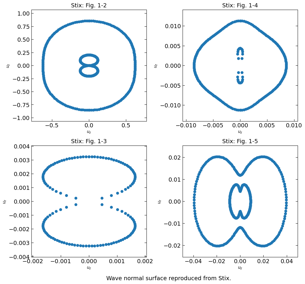
Here we can define the parameters for all the plots in Stix 1992 and then reproduce them in the same fashion.

# define inputs
inputs_2 = {
    "theta": np.linspace(0, np.pi, 100) * u.rad,
    "ions": Particle("p"),
    "n_i": 1e12 * u.cm**-3,
    "B": 0.434 * u.T,
    "w": (37125810) * u.rad / u.s,
}

inputs_3 = {
    "theta": np.linspace(0, np.pi, 100) * u.rad,
    "ions": Particle("p"),
    "n_i": 1e12 * u.cm**-3,
    "B": 0.434534 * u.T,
    "w": (2 * 10**10) * u.rad / u.s,
}

inputs_4 = {
    "theta": np.linspace(0, np.pi, 100) * u.rad,
    "ions": Particle("p"),
    "n_i": 1e12 * u.cm**-3,
    "B": 0.434600 * u.T,
    "w": (54 * 10**9) * u.rad / u.s,
}

inputs_5 = {
    "theta": np.linspace(0, np.pi, 100) * u.rad,
    "ions": Particle("p"),
    "n_i": 1e12 * u.cm**-3,
    "B": 0.434634 * u.T,
    "w": (58 * 10**9) * u.rad / u.s,
}

# define a list of all inputs
stix_inputs = [inputs_1, inputs_2, inputs_3, inputs_4, inputs_5]

Following on, the same method implemented on the first set of input parameters can be implemented on the rest. Afterwards, the result for all inputs can be plotted.

stix_plt = {}

ux = {}
uz = {}

for i in range(len(stix_inputs)):
    stix_plt[i] = {}


for i, inpt in enumerate(stix_inputs):
    omegas, thetas = np.meshgrid(inpt["w"].value, inpt["theta"].value, indexing="ij")
    omegas = np.dstack((omegas,) * 4).squeeze()
    thetas = np.dstack((thetas,) * 4).squeeze()

    k = stix(**inpt)

    mask = np.imag(k) == 0

    va = speeds.va_(inpt["B"], inpt["n_i"], ion=inpt["ions"])

    for arr in k:
        val = 0
        for item in arr:
            val = val + item**2
        norm = (np.sqrt(val) * va / inpt["w"]).value ** 2
        stix_plt[i] = {
            "ux": norm
            * omegas[mask]
            * np.sin(thetas[mask])
            / (k.value[mask] * c.value),
            "uz": norm
            * omegas[mask]
            * np.cos(thetas[mask])
            / (k.value[mask] * c.value),
        }

Plot the results.

# create figure
fig, axs = plt.subplots(2, 2, figsize=[figwidth, figheight])


for i in range(2):
    for j in range(2):
        axs[i, j].scatter(
            stix_plt[i + 2 * j + 1]["ux"], stix_plt[i + 2 * j + 1]["uz"], label="dfwd"
        )
        axs[i, j].set_title("Stix: Fig. 1-" + str(i + 2 * j + 2), fontsize=fs)

        # adjust axes
        axs[i, j].set(
            ylabel=r"$u_z$",
            xlabel=r"$u_z$",
        )

        pad = 1.25
        axs[i, j].set_ylim(
            min(stix_plt[i + 2 * j + 1]["uz"]) * pad,
            max(stix_plt[i + 2 * j + 1]["uz"]) * pad,
        )
        axs[i, j].set_xlim(
            min(stix_plt[i + 2 * j + 1]["ux"]) * pad,
            max(stix_plt[i + 2 * j + 1]["ux"]) * pad,
        )

        axs[i, j].tick_params(
            which="both",
            direction="in",
            labelsize=fs,
            right=True,
            length=5,
        )


# plot caption
txt = "Wave normal surface reproduced from Stix."

plt.tight_layout()
plt.figtext(0.35, -0.02, txt, ha="left", fontsize=fs)


plt.show()

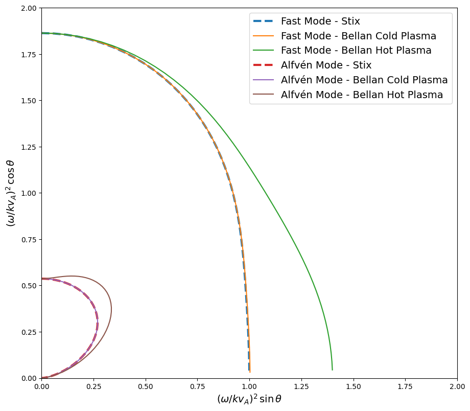
Comparison with Bellan

Below we run a comparison between the solution provided in Bellan 2012 and our own solutions computed from stix(). To begin we first create a function that reproduces the Bellan plot.

def norm_bellan_plot(**inputs):
    """Reproduce plot of Bellan dispersion relation."""
    w = inputs["w"]
    k = inputs["k"]
    theta = inputs["theta"]

    if w.shape == k.shape or w.size == 1 or k.size == 1:
        pass
    elif w.ndim > 2 or k.ndim > 2 or k.shape[0] != w.shape[0]:
        raise ValueError
    elif k.ndim > w.ndim:
        w = np.repeat(w[..., np.newaxis], k.shape[1], axis=1)
    elif k.ndim < w.ndim:
        k = np.repeat(k[..., np.newaxis], w.shape[1], axis=1)

    if theta.ndim != 1 or theta.size != w.shape[-1]:
        raise ValueError

    try:
        ion = inputs["ion"]
    except KeyError:
        ion = inputs["ions"][0]
    va = speeds.va_(inputs["B"], inputs["n_i"], ion=ion)

    mag = ((w / (k * va)).to(u.dimensionless_unscaled).value) ** 2
    theta = theta.to(u.radian).value

    xnorm = mag * np.sin(theta)
    ynorm = mag * np.cos(theta)

    return np.array([xnorm, ynorm])

Now we can solve the Bellan solution for identical plasma parameters, in the first instance a cold plasma limit of \(k_B T_e = 0.1\) eV and \(k_B T_p = 0.1\) eV are assumed. In the second instance a warm plasma limit of \(k_B T_e = 20\) eV and \(k_B T_p = 10\) eV are assumed.

# defining all inputs
base_inputs = {
    "k": (2 * np.pi * u.rad) / (0.56547 * u.m),
    "theta": np.linspace(0, 0.49 * np.pi, 50) * u.rad,
    "ion": Particle("He-4 1+"),
    "n_i": 6.358e19 * u.m**-3,
    "B": 400e-4 * u.T,
}

hot_inputs = {
    **base_inputs,
    "T_e": 20 * u.eV,
    "T_i": 10 * u.eV,
}

cold_inputs = {
    **base_inputs,
    "T_e": 0.1 * u.eV,
    "T_i": 0.1 * u.eV,
}

# calculating the solution from two fluid
w_tf_hot = two_fluid(**hot_inputs)
w_tf_cold = two_fluid(**cold_inputs)

plt_tf_hot = {}
for key, val in w_tf_hot.items():
    plt_tf_hot[key] = norm_bellan_plot(**{**hot_inputs, "w": val})

plt_tf_cold = {}
for key, val in w_tf_cold.items():
    plt_tf_cold[key] = norm_bellan_plot(**{**cold_inputs, "w": val})

Stix needs to recalculated using the Bellan inputs as a base.

stix_inputs = {**base_inputs, "ions": [base_inputs["ion"]]}
del stix_inputs["k"]
del stix_inputs["ion"]

Bellan fixes \(k\) and then calculates \(ω\) for each mode and propagation angle \(θ\). This means we cannot simply take solutions from Bellan and get corresponding \(k\) values via Stix. In order to solve this problem we need to create a version of stix() that can be optimized by scipy.optimize.root_scalar().

# partially bind plasma parameter keywords to stix()
_opt = stix_inputs.copy()
del _opt["theta"]
stix_partial = functools.partial(stix, **_opt)


def stix_optimize(w, theta, mode, k_expected):
    """Version of `stix` that can be optimized by `scipy.optimize.root_scalar`."""
    w = np.abs(w)
    results = stix_partial(w=w * u.rad / u.s, theta=theta * u.rad).value

    # only consider real and positive solutions
    real_mask = np.where(np.imag(results) == 0, True, False)
    pos_mask = np.where(np.real(results) > 0, True, False)
    mask = np.logical_and(real_mask, pos_mask)

    # get the correct k to compare
    if np.count_nonzero(mask) == 1:
        results = np.real(results[mask][0])
    elif mode == "fast_mode":
        # fast_mode has a larger phase velocity than
        # the alfven_mode, thus take the smaller k-value
        results = np.min(np.real(results[mask]))
    else:  # alfven_mode
        results = np.max(np.real(results[mask]))

    return results - k_expected

Let’s use the Cold case Bellan solution to solve for the Stix solution. Note only the fast_mode and slow_mode solutions are being used to seed the Stix solution because the acoustic_mode disappears in the cold plasma limit.

theta_arr = cold_inputs["theta"].value
k_expected = base_inputs["k"].value
k_stix = {}
w_stix = {}
for mode in ("fast_mode", "alfven_mode"):
    w_arr = w_tf_cold[mode].value
    k_stix[mode] = []
    w_stix[mode] = []
    for ii in range(w_arr.size):
        w_guess = w_arr[ii]
        _theta = theta_arr[ii]
        result = scipy.optimize.root_scalar(
            stix_optimize,
            args=(_theta, mode, k_expected),
            x0=w_guess,
            x1=w_guess + 1e2,
        )

        # append the wavefrequency (result.root) that
        # corresponded to stix() returning k_expected
        w_stix[mode].append(np.real(result.root))

        # double check and store the k-value
        _k = stix(
            **{
                **stix_inputs,
                "w": np.real(result.root) * u.rad / u.s,
                "theta": theta_arr[ii] * u.rad,
            }
        ).value
        real_mask = np.where(np.imag(_k) == 0, True, False)
        pos_mask = np.where(np.real(_k) > 0, True, False)
        mask = np.logical_and(real_mask, pos_mask)

        _k = np.real(_k[mask])
        mask = np.isclose(_k, base_inputs["k"].value)
        k_stix[mode].append(_k[mask][0])

    k_stix[mode] = np.array(k_stix[mode])
    w_stix[mode] = np.array(w_stix[mode])

(
    k_expected,
    k_stix,
    w_stix,
)

(11.111438815816198,
 {'fast_mode': array([11.11143882, 11.11143882, 11.11143882, 11.11143882, 11.11143882,
         11.11143882, 11.11143882, 11.11143882, 11.11143882, 11.11143882,
         11.11143882, 11.11143882, 11.11143882, 11.11143882, 11.11143882,
         11.11143882, 11.11143882, 11.11143882, 11.11143882, 11.11143882,
         11.11143882, 11.11143882, 11.11143882, 11.11143882, 11.11143882,
         11.11143882, 11.11143882, 11.11143882, 11.11143882, 11.11143882,
         11.11143882, 11.11143882, 11.11143882, 11.11143882, 11.11143882,
         11.11143882, 11.11143882, 11.11143882, 11.11143882, 11.11143882,
         11.11143882, 11.11143882, 11.11143882, 11.11143882, 11.11143882,
         11.11143882, 11.11143882, 11.11143882, 11.11143882, 11.11143882]),
  'alfven_mode': array([11.11143882, 11.11143882, 11.11143882, 11.11143882, 11.11143882,
         11.11143882, 11.11143882, 11.11143882, 11.11143882, 11.11143882,
         11.11143882, 11.11143882, 11.11143882, 11.11143882, 11.11143882,
         11.11143882, 11.11143882, 11.11143882, 11.11143882, 11.11143882,
         11.11143882, 11.11143882, 11.11143882, 11.11143882, 11.11143882,
         11.11143882, 11.11143882, 11.11143882, 11.11143882, 11.11143882,
         11.11143882, 11.11143882, 11.11143882, 11.11143882, 11.11143882,
         11.11143882, 11.11143882, 11.11143882, 11.11143882, 11.11143882,
         11.11143882, 11.11143882, 11.11143882, 11.11143882, 11.11143882,
         11.11143882, 11.11143882, 11.11143882, 11.11143882, 11.11143882])},
 {'fast_mode': array([832492.67093923, 832225.41983245, 831424.65541629, 830093.35115222,
         828236.48528083, 825861.07442708, 822976.22039535, 819593.16978312,
         815725.38575956, 811388.63092296, 806601.05952407, 801383.31646426,
         795758.6392925 , 789752.95787728, 783394.98447966, 776716.28459426,
         769751.31621087, 762537.42223423, 755114.75797978, 747526.1334238 ,
         739816.74892316, 732033.8043225 , 724225.96571732, 716442.68250546,
         708733.36014995, 701146.41085685, 693728.22349643, 686522.11261265,
         679567.3203566 , 672898.15064463, 666543.30895403, 660525.50346248,
         654861.33618235, 649561.48130428, 644631.11822484, 640070.56408932,
         635876.03837404, 632040.49056475, 628554.42948308, 625406.70603181,
         622585.21659703, 620077.50920212, 617871.28692075, 615954.81221471,
         614317.2217517 , 612948.76434044, 611840.97555855, 610986.80211157,
         610380.68751398, 610018.62874915]),
  'alfven_mode': array([446821.74544455, 446744.68217937, 446512.88191043, 446124.50625464,
         445576.46805747, 444864.39672569, 443982.5899558 , 442923.95223925,
         441679.92081177, 440240.38014901, 438593.56674162, 436725.96676382,
         434622.2104388 , 432264.96845572, 429634.85774751, 426710.36630245,
         423467.80940179, 419881.33259628, 415922.97955985, 411562.84520481,
         406769.33541317, 401509.55354398, 395749.82953427, 389456.39905716,
         382596.22742021, 375137.95611849, 367052.9308445 , 358316.2512548 ,
         348907.7688182 , 338812.95362154, 328023.55691657, 316538.0139173 ,
         304361.55843447, 291506.05239366, 277989.56304713, 263835.7433588 ,
         249073.08337343, 233734.10187313, 217854.54015126, 201472.60653188,
         184628.30480599, 167362.86489671, 149718.28163455, 131736.95832046,
         113461.4457862 ,  94934.26444988,  76197.79573168,  57294.2294464 ,
          38265.55483303,  19153.5842565 ])})

Create normalized arrays for plotting.

plt_stix = {}
for key, val in k_stix.items():
    plt_stix[key] = norm_bellan_plot(
        **{**stix_inputs, "k": val * u.rad / u.m, "w": w_stix[key] * u.rad / u.s}
    )

Plot the results.

fig = plt.figure(figsize=[figwidth, figheight])

mode = "fast_mode"
plt.plot(
    plt_stix[mode][0, ...],
    plt_stix[mode][1, ...],
    "--",
    linewidth=3,
    label="Fast Mode - Stix",
)
plt.plot(
    plt_tf_cold[mode][0, ...],
    plt_tf_cold[mode][1, ...],
    label="Fast Mode - Bellan Cold Plasma",
)
plt.plot(
    plt_tf_hot[mode][0, ...],
    plt_tf_hot[mode][1, ...],
    label="Fast Mode - Bellan Hot Plasma",
)

mode = "alfven_mode"
plt.plot(
    plt_stix[mode][0, ...],
    plt_stix[mode][1, ...],
    "--",
    linewidth=3,
    label="Alfvén Mode - Stix",
)
plt.plot(
    plt_tf_cold[mode][0, ...],
    plt_tf_cold[mode][1, ...],
    label="Alfvén Mode - Bellan Cold Plasma",
)
plt.plot(
    plt_tf_hot[mode][0, ...],
    plt_tf_hot[mode][1, ...],
    label="Alfvén Mode - Bellan Hot Plasma",
)

plt.legend(fontsize=fs)

plt.xlabel(r"$(ω / k v_A)^2 \, \sin θ$", fontsize=fs)
plt.ylabel(r"$(ω / k v_A)^2 \, \cos θ$", fontsize=fs)
plt.xlim(0.0, 2.0)
plt.ylim(0.0, 2.0);