This page was generated by
nbsphinx from
docs/notebooks/dispersion/two_fluid_dispersion.ipynb.
Interactive online version:
![]() .
.
Dispersion: A Full Two Fluid Solution
This notebook walks through the functionality of the two_fluid() function. This function computes the wave frequencies for given wavenumbers and plasma parameters based on the analytical solution presented by Bellan 2012 to the Stringer 1963 two fluid dispersion relation. The two fluid dispersion equation assumes a uniform magnetic field, a zero D.C. electric field, and low-frequency waves \(\omega / k c \ll 1\) which equates to
where
\(\omega\) is the wave frequency, \(k\) is the wavenumber, \(v_A\) is the Alfvén velocity, \(c_s\) is the sound speed, \(\omega_{ci}\) is the ion gyrofrequency, and \(\omega_{pe}\) is the electron plasma frequency.
The approach outlined in Section 5 of Bellan 2012 produces exact roots to the above dispersion equation for all three modes (fast, acoustic, and Alfvén) without having to make additional approximations. The following dispersion relation is what the two_fluid() function computes.
where \(j = 0\) represents the fast mode, \(j = 1\) represents the Alfvén mode, and \(j = 2\) represents the acoustic mode. Additionally,
Contents:
[1]:
%matplotlib inline

import astropy.units as u
import matplotlib.pyplot as plt
import numpy as np
from astropy.constants.si import c
from matplotlib.ticker import MultipleLocator
from mpl_toolkits.axes_grid1 import make_axes_locatable

from plasmapy.dispersion.analytical.two_fluid_ import two_fluid
from plasmapy.formulary import speeds
from plasmapy.formulary.frequencies import gyrofrequency, plasma_frequency, wc_, wp_
from plasmapy.formulary.lengths import inertial_length
from plasmapy.particles import Particle

plt.rcParams["figure.figsize"] = [10.5, 0.56 * 10.5]
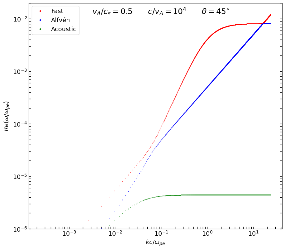
Wave Propagating at 45 Degrees
Below we define the required parameters to compute the wave frequencies.
[2]:
# define input parameters
inputs = {
    "k": np.linspace(10**-7, 10**-2, 10000) * u.rad / u.m,
    "theta": 45 * u.deg,
    "n_i": 5 * u.cm**-3,
    "B": 8.3e-9 * u.T,
    "T_e": 1.6e6 * u.K,
    "T_i": 4.0e5 * u.K,
    "ion": Particle("p+"),
}

# a few useful plasma parameters
params = {
    "n_e": inputs["n_i"] * abs(inputs["ion"].charge_number),
    "cs": speeds.ion_sound_speed(
        inputs["T_e"],
        inputs["T_i"],
        inputs["ion"],
    ),
    "va": speeds.Alfven_speed(
        inputs["B"],
        inputs["n_i"],
        ion=inputs["ion"],
    ),
    "wci": gyrofrequency(inputs["B"], inputs["ion"]),
}
params["lpe"] = inertial_length(params["n_e"], "e-")
params["wpe"] = plasma_frequency(params["n_e"], "e-")
The computed wave frequencies (\(rad/s\)) are returned in a dictionary with keys representing the wave modes and the values being an Astropy Quantity. Since our inputs had a scalar \(\theta\) and a 1D array of \(k\)’s, the computed wave frequencies will be a 1D array of size equal to the size of the \(k\) array.
[3]:
[3]:
(['fast_mode', 'alfven_mode', 'acoustic_mode'],
 <Quantity [1.63839709e-02, 1.80262570e-01, 3.44262572e-01, ...,
            1.52032171e+03, 1.52047365e+03, 1.52062560e+03] rad / s>,
 (10000,))
Let’s plot the results of each wave mode.
[4]:
fs = 14  # default font size
figwidth, figheight = plt.rcParams["figure.figsize"]
figheight = 1.6 * figheight
fig = plt.figure(figsize=[figwidth, figheight])

# normalize data
k_prime = inputs["k"] * params["lpe"]

# plot
plt.plot(
    k_prime,
    np.real(omegas["fast_mode"] / params["wpe"]),
    "r.",
    ms=1,
    label="Fast",
)
ax = plt.gca()
ax.plot(
    k_prime,
    np.real(omegas["alfven_mode"] / params["wpe"]),
    "b.",
    ms=1,
    label="Alfvén",
)
ax.plot(
    k_prime,
    np.real(omegas["acoustic_mode"] / params["wpe"]),
    "g.",
    ms=1,
    label="Acoustic",
)

# adjust axes
ax.set_xlabel(r"$kc / \omega_{pe}$", fontsize=fs)
ax.set_ylabel(r"$Re(\omega / \omega_{pe})$", fontsize=fs)
ax.set_yscale("log")
ax.set_xscale("log")
ax.set_ylim(1e-6, 2e-2)
ax.tick_params(
    which="both",
    direction="in",
    width=1,
    labelsize=fs,
    right=True,
    length=5,
)

# annotate
text = (
    rf"$v_A/c_s = {params['va'] / params['cs']:.1f} \qquad "
    rf"c/v_A = 10^{np.log10(c / params['va']):.0f} \qquad "
    f"\\theta = {inputs['theta'].value:.0f}"
    "^{\\circ}$"
)
ax.text(0.25, 0.95, text, transform=ax.transAxes, fontsize=18)
ax.legend(loc="upper left", markerscale=5, fontsize=fs)
[4]:
<matplotlib.legend.Legend at 0x73bf4b4f6ba0>
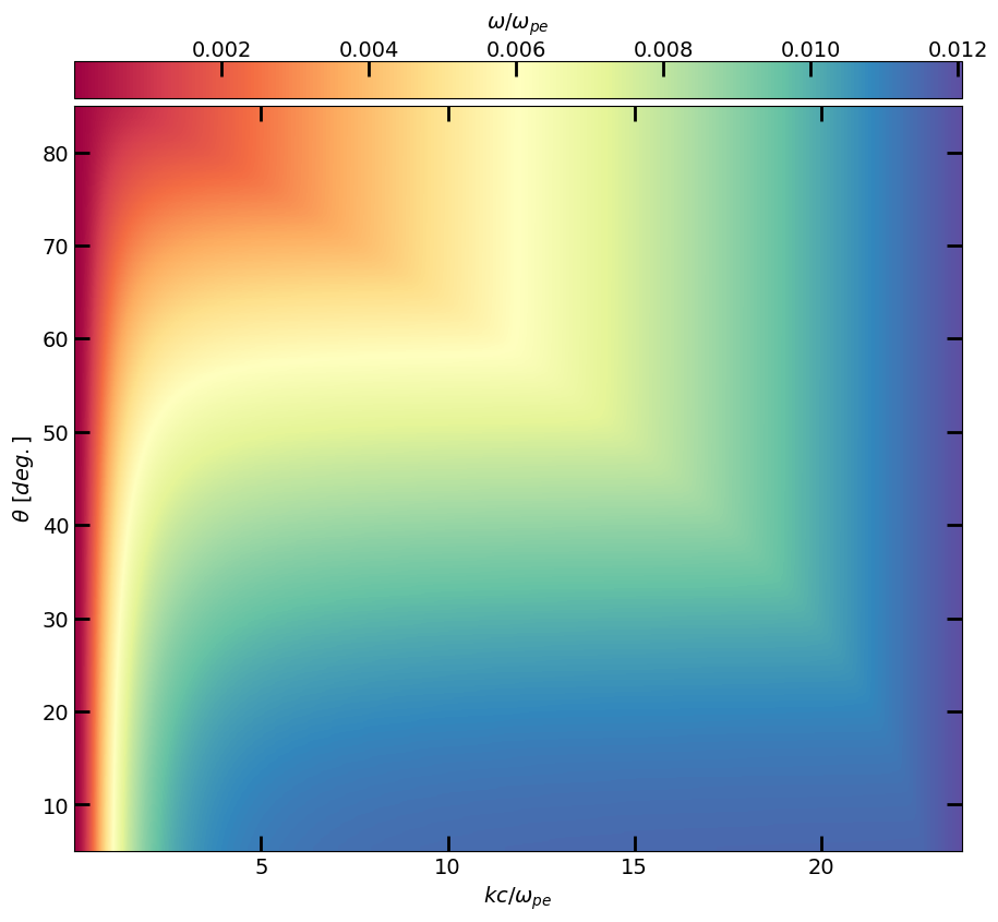
Wave frequencies on the k-theta plane
Let us now look at the distribution of \(\omega\) on a \(k\)-\(\theta\) plane.
[5]:
# define input parameters
inputs = {
    "k": np.linspace(10**-7, 10**-2, 10000) * u.rad / u.m,
    "theta": np.linspace(5, 85, 100) * u.deg,
    "n_i": 5 * u.cm**-3,
    "B": 8.3e-9 * u.T,
    "T_e": 1.6e6 * u.K,
    "T_i": 4.0e5 * u.K,
    "ion": Particle("p+"),
}

# a few useful plasma parameters
params = {
    "n_e": inputs["n_i"] * abs(inputs["ion"].charge_number),
    "cs": speeds.ion_sound_speed(
        inputs["T_e"],
        inputs["T_i"],
        inputs["ion"],
    ),
    "va": speeds.Alfven_speed(
        inputs["B"],
        inputs["n_i"],
        ion=inputs["ion"],
    ),
    "wci": gyrofrequency(inputs["B"], inputs["ion"]),
}
params["lpe"] = inertial_length(params["n_e"], "e-")
params["wpe"] = plasma_frequency(params["n_e"], "e-")
Since the \(\theta\) and \(k\) values are now 1-D arrays, the returned wave frequencies will be 2-D arrays with the first dimension matching the size of \(k\) and the second dimension matching the size of \(\theta\).
[6]:
# compute
omegas = two_fluid(**inputs)

(
    omegas["fast_mode"].shape,
    omegas["fast_mode"].shape[0] == inputs["k"].size,
    omegas["fast_mode"].shape[1] == inputs["theta"].size,
)
[6]:
((10000, 100), True, True)
Let’s plot (the fast mode)!
[7]:
fs = 14  # default font size
figwidth, figheight = plt.rcParams["figure.figsize"]
figheight = 1.6 * figheight
fig = plt.figure(figsize=[figwidth, figheight])

# normalize data
k_prime = inputs["k"] * params["lpe"]
zdata = np.transpose(np.real(omegas["fast_mode"].value)) / params["wpe"].value

# plot
im = plt.imshow(
    zdata,
    aspect="auto",
    origin="lower",
    extent=[
        np.min(k_prime.value),
        np.max(k_prime.value),
        np.min(inputs["theta"].value),
        np.max(inputs["theta"].value),
    ],
    interpolation=None,
    cmap=plt.cm.Spectral,
)
ax = plt.gca()

# # adjust axes
ax.set_xscale("linear")
ax.set_xlabel(r"$kc/\omega_{pe}$", fontsize=fs)
ax.set_ylabel(r"$\theta$ [$deg.$]", fontsize=fs)
ax.tick_params(
    which="both",
    direction="in",
    width=2,
    labelsize=fs,
    right=True,
    top=True,
    length=10,
)

# Add colorbar
divider = make_axes_locatable(ax)
cax = divider.append_axes("top", size="5%", pad=0.07)
cbar = plt.colorbar(
    im,
    cax=cax,
    orientation="horizontal",
    ticks=None,
    fraction=0.05,
    pad=0.0,
)
cbar.ax.tick_params(
    axis="x",
    direction="in",
    width=2,
    length=10,
    top=True,
    bottom=False,
    labelsize=fs,
    pad=0.0,
    labeltop=True,
    labelbottom=False,
)
cbar.ax.xaxis.set_label_position("top")
cbar.set_label(r"$\omega/\omega_{pe}$", fontsize=fs, labelpad=8)
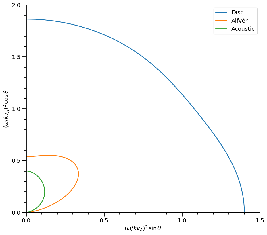
Reproduce Figure 1 from Bellan 2012
Figure 1 of Bellan 2012 chooses parameters such that \(\beta = 0.4\) and \(\Lambda=0.4\). Below we define parameters to approximate Bellan’s assumptions.
[8]:
# define input parameters
inputs = {
    "B": 400e-4 * u.T,
    "ion": Particle("He+"),
    "n_i": 6.358e19 * u.m**-3,
    "T_e": 20 * u.eV,
    "T_i": 10 * u.eV,
    "theta": np.linspace(0, 90) * u.deg,
    "k": (2 * np.pi * u.rad) / (0.56547 * u.m),
}

# a few useful plasma parameters
params = {
    "n_e": inputs["n_i"] * abs(inputs["ion"].charge_number),
    "cs": speeds.cs_(inputs["T_e"], inputs["T_i"], inputs["ion"]),
    "wci": wc_(inputs["B"], inputs["ion"]),
    "va": speeds.va_(inputs["B"], inputs["n_i"], ion=inputs["ion"]),
}
params["beta"] = (params["cs"] / params["va"]).value ** 2
params["wpe"] = wp_(params["n_e"], "e-")
params["Lambda"] = (inputs["k"] * params["va"] / params["wci"]).value ** 2

(params["beta"], params["Lambda"])
[8]:
(np.float64(0.4000832135717194), np.float64(0.4000017351804854))
[9]:
# compute
omegas = two_fluid(**inputs)
[10]:
# generate data for plots
plt_vals = {}
for mode, arr in omegas.items():
    norm = (np.absolute(arr) / (inputs["k"] * params["va"])).value ** 2
    plt_vals[mode] = {
        "x": norm * np.sin(inputs["theta"].to(u.rad).value),
        "y": norm * np.cos(inputs["theta"].to(u.rad).value),
    }
[11]:
fs = 14  # default font size
figwidth, figheight = plt.rcParams["figure.figsize"]
figheight = 1.6 * figheight
fig = plt.figure(figsize=[figwidth, figheight])

# Fast mode
plt.plot(
    plt_vals["fast_mode"]["x"],
    plt_vals["fast_mode"]["y"],
    linewidth=2,
    label="Fast",
)
ax = plt.gca()

# adjust axes
ax.set_xlabel(r"$(\omega / k v_A)^2 \, \sin \theta$", fontsize=fs)
ax.set_ylabel(r"$(\omega / k v_A)^2 \, \cos \theta$", fontsize=fs)
ax.set_xlim(0.0, 1.5)
ax.set_ylim(0.0, 2.0)
for spine in ax.spines.values():
    spine.set_linewidth(2)
ax.minorticks_on()
ax.tick_params(which="both", labelsize=fs, width=2)
ax.tick_params(which="major", length=10)
ax.tick_params(which="minor", length=5)
ax.xaxis.set_major_locator(MultipleLocator(0.5))
ax.xaxis.set_minor_locator(MultipleLocator(0.1))
ax.yaxis.set_major_locator(MultipleLocator(0.5))
ax.yaxis.set_minor_locator(MultipleLocator(0.1))


# Alfven mode
plt.plot(
    plt_vals["alfven_mode"]["x"],
    plt_vals["alfven_mode"]["y"],
    linewidth=2,
    label="Alfvén",
)

# Acoustic mode
plt.plot(
    plt_vals["acoustic_mode"]["x"],
    plt_vals["acoustic_mode"]["y"],
    linewidth=2,
    label="Acoustic",
)

# annotations
plt.legend(fontsize=fs, loc="upper right")
[11]:
<matplotlib.legend.Legend at 0x73bf4873ee40>