This page was generated by nbsphinx from docs/notebooks/dispersion/dispersion_function.ipynb.
Interactive online version: Binder badge.

[1]:
%matplotlib inline

The plasma dispersion function

Let’s import some basics (and PlasmaPy!)

[2]:
import matplotlib.pyplot as plt
import numpy as np
Help on function plasma_dispersion_func in module plasmapy.dispersion.dispersionfunction:

plasma_dispersion_func(zeta: Union[complex, numpy.ndarray, astropy.units.quantity.Quantity]) -> Union[complex, numpy.ndarray, astropy.units.quantity.Quantity]
    Calculate the plasma dispersion function.

    Parameters
    ----------
    zeta : complex, int, float, ~numpy.ndarray, or ~astropy.units.Quantity
        Argument of plasma dispersion function.

    Returns
    -------
    Z : complex, float, or ~numpy.ndarray
        Value of plasma dispersion function.

    Raises
    ------
    TypeError
        If the argument is of an invalid type.

    ~astropy.units.UnitsError
        If the argument is a `~astropy.units.Quantity` but is not
        dimensionless.

    ValueError
        If the argument is not entirely finite.

    See Also
    --------
    plasma_dispersion_func_deriv

    Notes
    -----
    The plasma dispersion function is defined as:

    .. math::
        Z(\zeta) = \pi^{-0.5} \int_{-\infty}^{+\infty}
        \frac{e^{-x^2}}{x-\zeta} dx

    where the argument is a complex number :cite:p:`fried:1961`.

    In plasma wave theory, the plasma dispersion function appears
    frequently when the background medium has a Maxwellian
    distribution function.  The argument of this function then refers
    to the ratio of a wave's phase velocity to a thermal velocity.

    Examples
    --------
    >>> plasma_dispersion_func(0)
    1.7724538509055159j
    >>> plasma_dispersion_func(1j)
    0.757872156141312j
    >>> plasma_dispersion_func(-1.52+0.47j)
    (0.6088888957234254+0.33494583882874024j)

    For user convenience
    `~plasmapy.dispersion.dispersionfunction.plasma_dispersion_func_lite`
    is bound to this function and can be used as follows:

    >>> plasma_dispersion_func.lite(0)
    1.7724538509055159j
    >>> plasma_dispersion_func.lite(1j)
    0.757872156141312j
    >>> plasma_dispersion_func.lite(-1.52+0.47j)
    (0.6088888957234254+0.33494583882874024j)

Take a look at the docs to plasma_dispersion_func() for more information on this.

We’ll now make some sample data to visualize the dispersion function:

[4]:
x = np.linspace(-1, 1, 1000)
X, Y = np.meshgrid(x, x)
Z = X + 1j * Y
print(Z.shape)
(1000, 1000)

Before we start plotting, let’s make a visualization function first:

[5]:
def plot_complex(X, Y, Z, N=50):
    fig, (real_axis, imag_axis) = plt.subplots(1, 2)
    real_axis.contourf(X, Y, Z.real, N)
    imag_axis.contourf(X, Y, Z.imag, N)
    real_axis.set_title("Real values")
    imag_axis.set_title("Imaginary values")
    for ax in [real_axis, imag_axis]:
        ax.set_xlabel("Real values")
        ax.set_ylabel("Imaginary values")
    fig.tight_layout()


plot_complex(X, Y, Z)
../../_images/notebooks_dispersion_dispersion_function_8_0.png

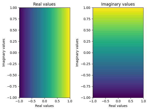
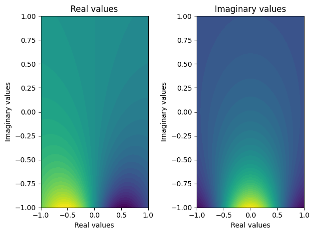
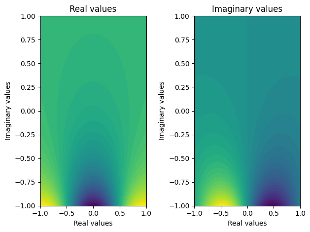
We can now apply our visualization function to our simple dispersion relation

[6]:
# sphinx_gallery_thumbnail_number = 2
F = plasmapy.dispersion.dispersionfunction.plasma_dispersion_func(Z)
plot_complex(X, Y, F)
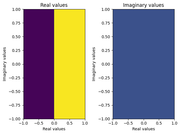
../../_images/notebooks_dispersion_dispersion_function_10_0.png

So this is going to be a hack and I’m not 100% sure the dispersion function is quite what I think it is, but let’s find the area where the dispersion function has a lesser than zero real part because I think it may be important (brb reading Fried and Conte):

[7]:
plot_complex(X, Y, F.real < 0)
../../_images/notebooks_dispersion_dispersion_function_12_0.png

We can also visualize the derivative:

../../_images/notebooks_dispersion_dispersion_function_14_0.png

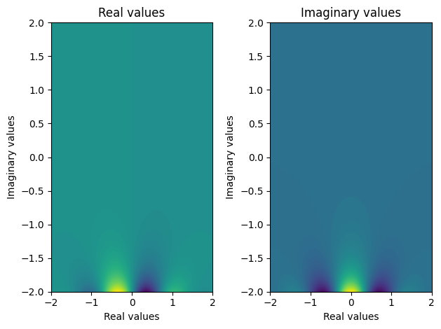
Plotting the same function on a larger area:

[9]:
x = np.linspace(-2, 2, 2000)
X, Y = np.meshgrid(x, x)
Z = X + 1j * Y
print(Z.shape)
(2000, 2000)
[10]:
../../_images/notebooks_dispersion_dispersion_function_17_0.png

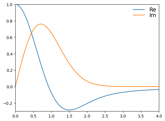
Now we examine the derivative of the dispersion function as a function of the phase velocity of an electromagnetic wave propagating through the plasma. This is recreating figure 5.1 in: J. Sheffield, D. Froula, S. H. Glenzer, and N. C. Luhmann Jr, Plasma scattering of electromagnetic radiation: theory and measurement techniques. Chapter 5 Pg 106 (Academic press, 2010).

[11]:
xs = np.linspace(0, 4, 100)
ws = (-1 / 2) * plasmapy.dispersion.dispersionfunction.plasma_dispersion_func_deriv(xs)
wRe = np.real(ws)
wIm = np.imag(ws)

plt.plot(xs, wRe, label="Re")
plt.plot(xs, wIm, label="Im")
plt.axis([0, 4, -0.3, 1])
plt.legend(
    loc="upper right", frameon=False, labelspacing=0.001, fontsize=14, borderaxespad=0.1
)
plt.show()
../../_images/notebooks_dispersion_dispersion_function_19_0.png