This page was generated by
nbsphinx from
docs/notebooks/dispersion/hollweg_dispersion.ipynb.
Interactive online version:
![]() .
.
Hollweg Dispersion Solver
This notebook details the functionality of the hollweg() function. This function computes the wave frequencies for given wavenumbers and plasma parameters based on the solution to the two fluid dispersion relation presented by Hollweg 1999, and further summarized by Bellan 2012. In his derivation Hollweg assumed a uniform magnetic field, zero D.C electric field, quasi-neutrality, and low-frequency waves (\(\omega \ll \omega_{ci}\)), which yielded the following expression
where
\(\omega\) is the wave frequency, \(k\) is the wavenumber , \(v_{A}\) is the Alfvén velocity, \(c_{s}\) is the ion sound speed, \(\omega_{ci}\) is the ion gyrofrequency, and \(\omega_{pe}\) is the electron plasma frequency.
Note
Hollweg 1999 asserts this expression is valid for arbitrary \(c_{s} / v_{A}\) and \(k_{z} / k\). Contrarily, Bellan 2012 states in Section 1.7 that due to the inconsistent retention of the \(\omega / \omega_{ci} \ll 1\) terms the expression can only be valid if both \(c_{s} \ll v_{A}\) and the wave propagation is nearly perpendicular to the magnetic field (\(|\theta - \pi/2| \ll 0.1\) radians).
The hollweg() function numerically solves for the roots of this equation, which correspond to the Fast, Alfvén, and Acoustic wave modes.
Contents:
[1]:
%matplotlib inline

import warnings

import astropy.units as u
import matplotlib.pyplot as plt
import numpy as np
from matplotlib.ticker import MultipleLocator

from plasmapy.dispersion.analytical.two_fluid_ import two_fluid
from plasmapy.dispersion.numerical.hollweg_ import hollweg
from plasmapy.formulary import (
    Alfven_speed,
    gyrofrequency,
    inertial_length,
    ion_sound_speed,
    plasma_frequency,
)
from plasmapy.particles import Particle
from plasmapy.utils.exceptions import PhysicsWarning

warnings.filterwarnings(
    action="ignore",
    category=PhysicsWarning,
    module="plasmapy.dispersion.numerical.hollweg_",
)

plt.rcParams["figure.figsize"] = [10.5, 0.56 * 10.5]
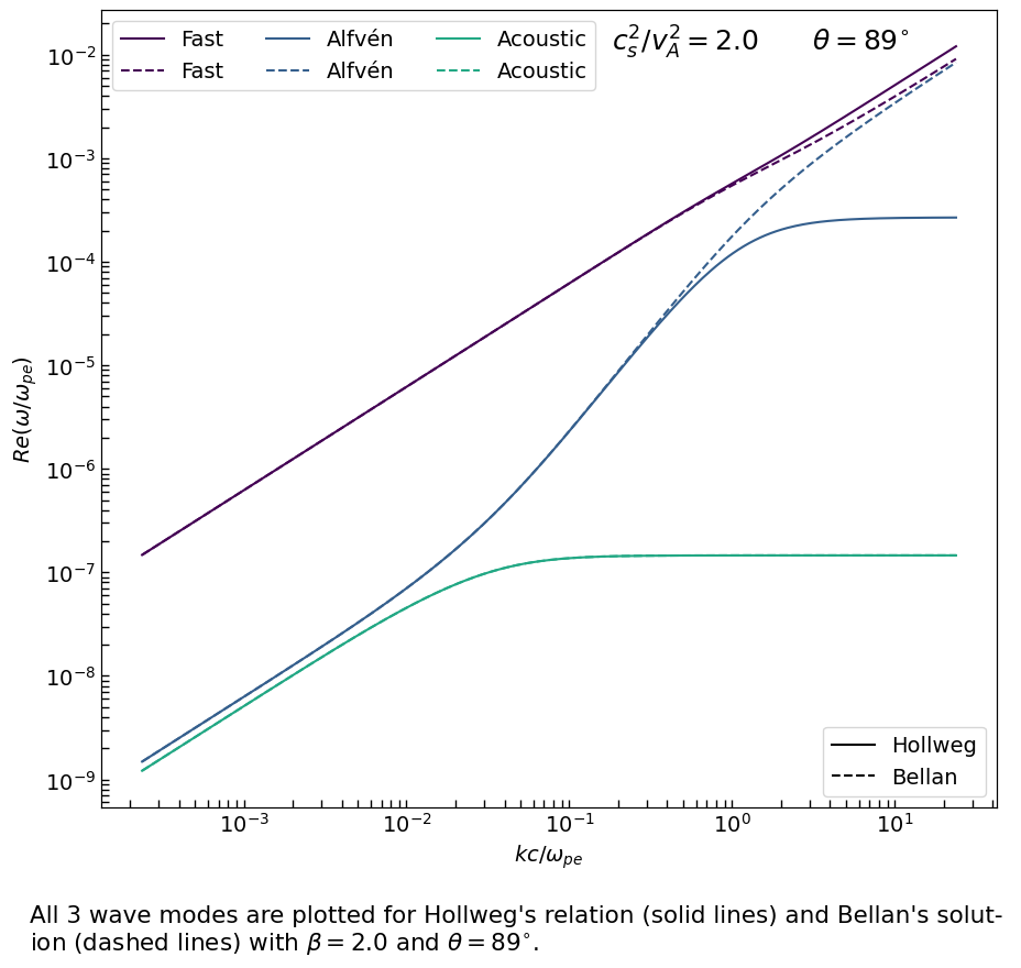
Wave propagating at nearly 90 degrees
Below we define the required parameters to compute the wave frequencies.
[2]:
# define input parameters
inputs = {
    "k": np.logspace(-7, -2, 300) * u.rad / u.m,
    "theta": 89 * u.deg,
    "n_i": 5 * u.cm**-3,
    "B": 1.10232e-8 * u.T,
    "T_e": 1.6e6 * u.K,
    "T_i": 4.0e5 * u.K,
    "ion": Particle("p+"),
}

# a few useful plasma parameters
params = {
    "n_e": inputs["n_i"] * abs(inputs["ion"].charge_number),
    "cs": ion_sound_speed(
        inputs["T_e"],
        inputs["T_i"],
        inputs["ion"],
    ),
    "va": Alfven_speed(
        inputs["B"],
        inputs["n_i"],
        ion=inputs["ion"],
    ),
    "wci": gyrofrequency(inputs["B"], inputs["ion"]),
}
params["lpe"] = inertial_length(params["n_e"], "e-")
params["wpe"] = plasma_frequency(params["n_e"], "e-")

# compute
omegas1 = hollweg(**inputs)
omegas2 = two_fluid(**inputs)
np.set_printoptions(precision=4, threshold=20)
/home/docs/checkouts/readthedocs.org/user_builds/plasmapy/checkouts/latest/src/plasmapy/particles/decorators.py:1009: PhysicsWarning: The Hollweg dispersion solver is valid the low beta regime: c_s / v_A ≪ 1 (see §1.7 of Bellan 2012, doi: 10.1029/2012ja017856). However, c_s / V_A = 1.41, which may affect the validity of the solution.
  return callable__(
/home/docs/checkouts/readthedocs.org/user_builds/plasmapy/checkouts/latest/src/plasmapy/particles/decorators.py:1009: PhysicsWarning: The Hollweg dispersion solver is valid in the regime where ω / ω_ci ≪ 1. However, the maximum value of ω / ω_ci for the solution is 1088.94+0.00j, which may affect the validity of the solution.
  return callable__(
The computed wave frequencies (rad/s) are returned in a dictionary with the keys representing wave modes and the values (instances of Astropy Quantity) being the frequencies. Since our inputs were a 1D arrays of of \(k\)’s, the computed wave frequencies will be a 1D array of size equal to the size of the \(k\) array.
[3]:
(list(omegas1.keys()), omegas1["fast_mode"], omegas1["fast_mode"].shape)
[3]:
(['fast_mode', 'alfven_mode', 'acoustic_mode'],
 <Quantity [1.8619e-02+0.j, 1.9350e-02+0.j, 2.0109e-02+0.j, ...,
            1.0663e+03+0.j, 1.1072e+03+0.j, 1.1498e+03+0.j] rad / s>,
 (300,))
Let’s plot the results of each wave mode.
[4]:
fs = 14  # default font size
figwidth, figheight = plt.rcParams["figure.figsize"]
figheight = 1.6 * figheight
fig = plt.figure(figsize=[figwidth, figheight])

# normalize data
k_prime = inputs["k"] * params["lpe"]

# define colormap
cmap = plt.get_cmap("viridis")
slicedCM = cmap(np.linspace(0, 0.6, 3))

# plot
(p1,) = plt.plot(
    k_prime,
    np.real(omegas1["fast_mode"] / params["wpe"]),
    "--",
    c=slicedCM[0],
    ms=1,
    label="Fast",
)
ax = plt.gca()
(p2,) = ax.plot(
    k_prime,
    np.real(omegas1["alfven_mode"] / params["wpe"]),
    "--",
    c=slicedCM[1],
    ms=1,
    label="Alfvén",
)
(p3,) = ax.plot(
    k_prime,
    np.real(omegas1["acoustic_mode"] / params["wpe"]),
    "--",
    c=slicedCM[2],
    ms=1,
    label="Acoustic",
)
(p4,) = plt.plot(
    k_prime,
    np.real(omegas2["fast_mode"] / params["wpe"]),
    c=slicedCM[0],
    ms=1,
    label="Fast",
)
ax = plt.gca()
(p5,) = ax.plot(
    k_prime,
    np.real(omegas2["alfven_mode"] / params["wpe"]),
    c=slicedCM[1],
    ms=1,
    label="Alfvén",
)
(p6,) = ax.plot(
    k_prime,
    np.real(omegas2["acoustic_mode"] / params["wpe"]),
    c=slicedCM[2],
    ms=1,
    label="Acoustic",
)

# adjust axes
ax.set_xlabel(r"$kc / \omega_{pe}$", fontsize=fs)
ax.set_ylabel(r"$Re(\omega / \omega_{pe})$", fontsize=fs)
ax.set_yscale("log")
ax.set_xscale("log")
ax.tick_params(
    which="both",
    direction="in",
    width=1,
    labelsize=fs,
    right=True,
    length=5,
)

# annotate
styles = ["-", "--"]
s_labels = ["Hollweg", "Bellan"]
ax2 = ax.twinx()
for ss, lab in enumerate(styles):
    ax2.plot(np.nan, np.nan, ls=lab, label=s_labels[ss], c="black")
ax2.get_yaxis().set_visible(False)
ax2.legend(fontsize=14, loc="lower right")

text1 = (
    rf"$c_s^2/v_A^2 = {params['cs'] ** 2 / params['va'] ** 2:.1f} \qquad "
    f"\\theta = {inputs['theta'].value:.0f}"
    "^{\\circ}$"
)
text2 = (
    "All 3 wave modes are plotted for Hollweg's relation (solid lines) and Bellan's solut- \n"
    f"ion (dashed lines) with $\\beta = 2.0$ and $\\theta = {inputs['theta'].value:.0f}"
    "^{\\circ}$."
)
plt.figtext(-0.08, -0.18, text2, ha="left", transform=ax.transAxes, fontsize=15.5)
ax.text(0.57, 0.95, text1, transform=ax.transAxes, fontsize=18)
ax.legend(handles=[p4, p1, p5, p2, p6, p3], fontsize=14, ncol=3, loc="upper left")
[4]:
<matplotlib.legend.Legend at 0x7f03b06738c0>
Hollweg 1999 and Bellan 2012 comparison
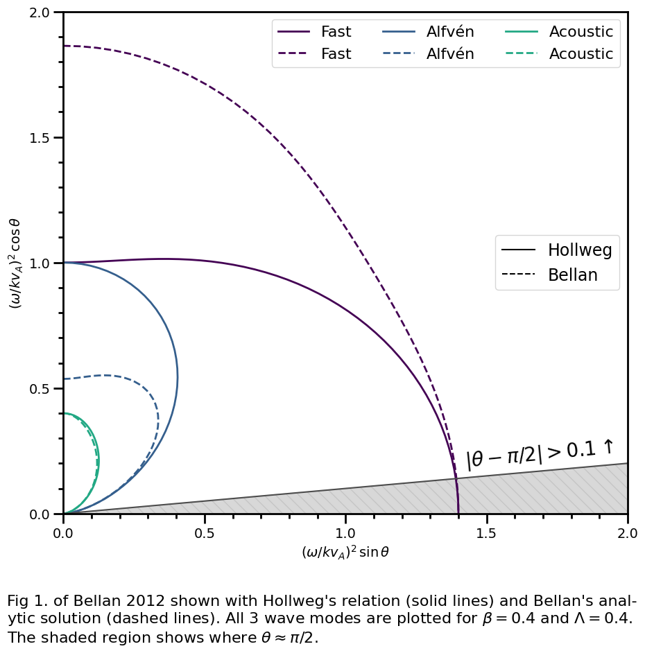
Figure 1 of Bellan 2012 chooses parameters such that \(\beta = 0.4\) and \(\Lambda = 0.4\). Below we define parameters to approximate Bellan’s assumptions.
[5]:
# define input parameters
inputs = {
    "B": 400e-4 * u.T,
    "ion": Particle("He+"),
    "n_i": 6.358e19 * u.m**-3,
    "T_e": 20 * u.eV,
    "T_i": 10 * u.eV,
    "theta": np.linspace(0, 90) * u.deg,
    "k": (2 * np.pi * u.rad) / (0.56547 * u.m),
}

# a few useful plasma parameters
params = {
    "n_e": inputs["n_i"] * abs(inputs["ion"].charge_number),
    "cs": ion_sound_speed(inputs["T_e"], inputs["T_i"], inputs["ion"]),
    "wci": gyrofrequency(inputs["B"], inputs["ion"]),
    "va": Alfven_speed(inputs["B"], inputs["n_i"], ion=inputs["ion"]),
}
params["beta"] = (params["cs"] / params["va"]).value ** 2
params["wpe"] = plasma_frequency(params["n_e"], "e-")
params["Lambda"] = (inputs["k"] * params["va"] / params["wci"]).value ** 2

(params["beta"], params["Lambda"])
[5]:
(np.float64(0.4000832135717194), np.float64(0.4000017351804854))
[6]:
/home/docs/checkouts/readthedocs.org/user_builds/plasmapy/checkouts/latest/src/plasmapy/particles/decorators.py:1009: PhysicsWarning: The Hollweg dispersion solver is valid the low beta regime: c_s / v_A ≪ 1 (see §1.7 of Bellan 2012, doi: 10.1029/2012ja017856). However, c_s / V_A = 0.63, which may affect the validity of the solution.
  return callable__(
/home/docs/checkouts/readthedocs.org/user_builds/plasmapy/checkouts/latest/src/plasmapy/particles/decorators.py:1009: PhysicsWarning: The Hollweg dispersion solver is valid in the regime where propagation is nearly perpendicular to the magnetic field (see §1.7 of Bellan 2012, doi: 10.1029/2012ja017856). However, a |θ - π/2| value of 1.57 was calculated, which may affect the validity of the solution.
  return callable__(
/home/docs/checkouts/readthedocs.org/user_builds/plasmapy/checkouts/latest/src/plasmapy/particles/decorators.py:1009: PhysicsWarning: The Hollweg dispersion solver is valid in the regime where ω / ω_ci ≪ 1. However, the maximum value of ω / ω_ci for the solution is 0.75+0.00j, which may affect the validity of the solution.
  return callable__(
[7]:
# generate data for Bellan curves
bellan_plt_vals = {}
for mode, arr in bellan_omegas.items():
    norm = (np.absolute(arr) / (inputs["k"] * params["va"])).value ** 2
    bellan_plt_vals[mode] = {
        "x": norm * np.sin(inputs["theta"].to(u.rad).value),
        "y": norm * np.cos(inputs["theta"].to(u.rad).value),
    }

# generate data for Hollweg curves
hollweg_plt_vals = {}
for mode, arr in hollweg_omegas.items():
    norm = (np.absolute(arr) / (inputs["k"] * params["va"])).value ** 2
    hollweg_plt_vals[mode] = {
        "x": norm * np.sin(inputs["theta"].to(u.rad).value),
        "y": norm * np.cos(inputs["theta"].to(u.rad).value),
    }
Let’s plot all 3 wave modes
[8]:
fs = 14  # default font size
figwidth, figheight = plt.rcParams["figure.figsize"]
figheight = 1.6 * figheight
fig = plt.figure(figsize=[figwidth, figheight])

# define colormap
cmap = plt.get_cmap("viridis")
slicedCM = cmap(np.linspace(0, 0.6, 3))

# Bellan Fast mode
(p1,) = plt.plot(
    bellan_plt_vals["fast_mode"]["x"],
    bellan_plt_vals["fast_mode"]["y"],
    "--",
    c=slicedCM[0],
    linewidth=2,
    label="Fast",
)
ax = plt.gca()

# adjust axes
ax.set_xlabel(r"$(\omega / k v_{A})^{2} \, \sin \theta$", fontsize=fs)
ax.set_ylabel(r"$(\omega / k v_{A})^{2} \, \cos \theta$", fontsize=fs)
ax.set_xlim(0.0, 2.0)
ax.set_ylim(0.0, 2.0)
for spine in ax.spines.values():
    spine.set_linewidth(2)
ax.minorticks_on()
ax.tick_params(which="both", labelsize=fs, width=2)
ax.tick_params(which="major", length=10)
ax.tick_params(which="minor", length=5)
ax.xaxis.set_major_locator(MultipleLocator(0.5))
ax.xaxis.set_minor_locator(MultipleLocator(0.1))
ax.yaxis.set_major_locator(MultipleLocator(0.5))
ax.yaxis.set_minor_locator(MultipleLocator(0.1))

# Bellan Alfven mode
(p2,) = plt.plot(
    bellan_plt_vals["alfven_mode"]["x"],
    bellan_plt_vals["alfven_mode"]["y"],
    "--",
    c=slicedCM[1],
    linewidth=2,
    label="Alfvén",
)

# Bellan Acoustic mode
(p3,) = plt.plot(
    bellan_plt_vals["acoustic_mode"]["x"],
    bellan_plt_vals["acoustic_mode"]["y"],
    "--",
    c=slicedCM[2],
    linewidth=2,
    label="Acoustic",
)

# Hollweg Fast mode
(p4,) = plt.plot(
    hollweg_plt_vals["fast_mode"]["x"],
    hollweg_plt_vals["fast_mode"]["y"],
    c=slicedCM[0],
    linewidth=2,
    label="Fast",
)

# Hollweg Alfven mode
(p5,) = plt.plot(
    hollweg_plt_vals["alfven_mode"]["x"],
    hollweg_plt_vals["alfven_mode"]["y"],
    c=slicedCM[1],
    linewidth=2,
    label="Alfvén",
)

# Hollweg Acoustic mode
(p6,) = plt.plot(
    hollweg_plt_vals["acoustic_mode"]["x"],
    hollweg_plt_vals["acoustic_mode"]["y"],
    c=slicedCM[2],
    linewidth=2,
    label="Acoustic",
)

# annotations
r = np.linspace(0, 2, 200)
X = (r**2) * np.cos(0.1)
Y = (r**2) * np.sin(0.1)
plt.plot(X, Y, color="0.3")
ax.fill_between(X, 0, Y, hatch="\\\\", color="0.7", alpha=0.5)

# style legend
styles = ["-", "--"]
s_labels = ["Hollweg", "Bellan"]
ax2 = ax.twinx()
for ss, lab in enumerate(styles):
    ax2.plot(np.nan, np.nan, ls=lab, label=s_labels[ss], c="black")
ax2.get_yaxis().set_visible(False)
ax2.legend(fontsize=17, loc="center right")

ax.legend(handles=[p4, p1, p5, p2, p6, p3], fontsize=16, ncol=3, loc="upper right")
plt.figtext(
    1.42,
    0.19,
    "$|\\theta - \\pi / 2| > 0.1 \\uparrow$",
    rotation=5.5,
    fontsize=20,
    transform=ax.transData,
)

# plot caption
txt = (
    "Fig 1. of Bellan 2012 shown with Hollweg's relation (solid lines) and Bellan's anal-\n"
    "ytic solution (dashed lines). All 3 wave modes are plotted for $\\beta= 0.4$ and $\\Lambda= 0.4$.\n"
    "The shaded region shows where $\\theta \\approx \\pi / 2$.\n"
)

plt.figtext(-0.1, -0.29, txt, ha="left", transform=ax.transAxes, fontsize=16);
Reproduce Figure 2 from Hollweg 1999
Figure 2 of Hollweg 1999 plots the Alfvén mode and chooses parameters such that \(\beta = 1/20, 1/2, 2, 1/2000\). Below we define parameters to approximate these values.
[9]:
# define input parameters
# beta = 1/20
inputs0 = {
    "k": np.logspace(-7, -2, 400) * u.rad / u.m,
    "theta": 90 * u.deg,
    "n_i": 5 * u.cm**-3,
    "B": 6.971e-8 * u.T,
    "T_e": 1.6e6 * u.K,
    "T_i": 4.0e5 * u.K,
    "ion": Particle("p+"),
}
# beta = 1/2
inputs1 = {
    **inputs0,
    "B": 2.205e-8 * u.T,
}
# beta = 2
inputs2 = {
    **inputs0,
    "B": 1.10232e-8 * u.T,
}
# beta = 1/2000
inputs3 = {
    **inputs0,
    "B": 6.97178e-7 * u.T,
}

# a few useful plasma parameters

# parameters corresponding to inputs0
params0 = {
    "n_e": inputs0["n_i"] * abs(inputs0["ion"].charge_number),
    "cs": ion_sound_speed(
        inputs0["T_e"],
        inputs0["T_i"],
        inputs0["ion"],
    ),
    "va": Alfven_speed(
        inputs0["B"],
        inputs0["n_i"],
        ion=inputs0["ion"],
    ),
    "wci": gyrofrequency(inputs0["B"], inputs0["ion"]),
}
params0["lpe"] = inertial_length(params0["n_e"], "e-")
params0["wpe"] = plasma_frequency(params0["n_e"], "e-")
params0["L"] = params0["cs"] / abs(params0["wci"])

# parameters corresponding to inputs1
params1 = {
    "n_e": inputs1["n_i"] * abs(inputs1["ion"].charge_number),
    "cs": ion_sound_speed(
        inputs1["T_e"],
        inputs1["T_i"],
        inputs1["ion"],
    ),
    "va": Alfven_speed(
        inputs1["B"],
        inputs1["n_i"],
        ion=inputs1["ion"],
    ),
    "wci": gyrofrequency(inputs1["B"], inputs1["ion"]),
}
params1["lpe"] = inertial_length(params1["n_e"], "e-")
params1["wpe"] = plasma_frequency(params1["n_e"], "e-")
params1["L"] = params1["cs"] / abs(params1["wci"])

# parameters corresponding to inputs2
params2 = {
    "n_e": inputs2["n_i"] * abs(inputs2["ion"].charge_number),
    "cs": ion_sound_speed(
        inputs2["T_e"],
        inputs2["T_i"],
        inputs2["ion"],
    ),
    "va": Alfven_speed(
        inputs2["B"],
        inputs2["n_i"],
        ion=inputs2["ion"],
    ),
    "wci": gyrofrequency(inputs2["B"], inputs2["ion"]),
}
params2["lpe"] = inertial_length(params2["n_e"], "e-")
params2["wpe"] = plasma_frequency(params2["n_e"], "e-")
params2["L"] = params2["cs"] / abs(params2["wci"])

# parameters corresponding to inputs3
params3 = {
    "n_e": inputs3["n_i"] * abs(inputs3["ion"].charge_number),
    "cs": ion_sound_speed(
        inputs3["T_e"],
        inputs3["T_i"],
        inputs3["ion"],
    ),
    "va": Alfven_speed(
        inputs3["B"],
        inputs3["n_i"],
        ion=inputs3["ion"],
    ),
    "wci": gyrofrequency(inputs3["B"], inputs3["ion"]),
}
params3["lpe"] = inertial_length(params3["n_e"], "e-")
params3["wpe"] = plasma_frequency(params3["n_e"], "e-")
params3["L"] = params3["cs"] / abs(params3["wci"])

# confirm beta values
beta_vals = [
    (params0["cs"] / params0["va"]).value ** 2,
    (params1["cs"] / params1["va"]).value ** 2,
    (params2["cs"] / params2["va"]).value ** 2,
    (params3["cs"] / params3["va"]).value ** 2,
]
print(
    f"1/{1 / beta_vals[0]:.4f}, "
    f"1/{1 / beta_vals[1]:.4f}, "
    f"{beta_vals[2]:.4f}, "
    f"1/{1 / beta_vals[3]:.4f}",
)
1/19.9955, 1/2.0006, 2.0001, 1/1999.9987
Figure 2 of Hollweg 1999 plots over some values that lie outside the valid regime which results in the PhysicsWarning’s below being raised.
[10]:
# compute omegas

# show warnings once
with warnings.catch_warnings():
    warnings.filterwarnings("once")
    omegas0 = hollweg(**inputs0)

omegas1 = hollweg(**inputs1)
omegas2 = hollweg(**inputs2)
omegas3 = hollweg(**inputs3)
/home/docs/checkouts/readthedocs.org/user_builds/plasmapy/checkouts/latest/src/plasmapy/particles/decorators.py:1009: PhysicsWarning: The Hollweg dispersion solver is valid the low beta regime: c_s / v_A ≪ 1 (see §1.7 of Bellan 2012, doi: 10.1029/2012ja017856). However, c_s / V_A = 0.22, which may affect the validity of the solution.
  return callable__(
/home/docs/checkouts/readthedocs.org/user_builds/plasmapy/checkouts/latest/src/plasmapy/particles/decorators.py:1009: PhysicsWarning: The Hollweg dispersion solver is valid in the regime where ω / ω_ci ≪ 1. However, the maximum value of ω / ω_ci for the solution is 1018.12+0.00j, which may affect the validity of the solution.
  return callable__(
/home/docs/checkouts/readthedocs.org/user_builds/plasmapy/checkouts/latest/src/plasmapy/particles/decorators.py:1009: PhysicsWarning: The Hollweg dispersion solver is valid the low beta regime: c_s / v_A ≪ 1 (see §1.7 of Bellan 2012, doi: 10.1029/2012ja017856). However, c_s / V_A = 0.71, which may affect the validity of the solution.
  return callable__(
/home/docs/checkouts/readthedocs.org/user_builds/plasmapy/checkouts/latest/src/plasmapy/particles/decorators.py:1009: PhysicsWarning: The Hollweg dispersion solver is valid in the regime where ω / ω_ci ≪ 1. However, the maximum value of ω / ω_ci for the solution is 1018.53+0.00j, which may affect the validity of the solution.
  return callable__(
/home/docs/checkouts/readthedocs.org/user_builds/plasmapy/checkouts/latest/src/plasmapy/particles/decorators.py:1009: PhysicsWarning: The Hollweg dispersion solver is valid the low beta regime: c_s / v_A ≪ 1 (see §1.7 of Bellan 2012, doi: 10.1029/2012ja017856). However, c_s / V_A = 1.41, which may affect the validity of the solution.
  return callable__(
/home/docs/checkouts/readthedocs.org/user_builds/plasmapy/checkouts/latest/src/plasmapy/particles/decorators.py:1009: PhysicsWarning: The Hollweg dispersion solver is valid in the regime where ω / ω_ci ≪ 1. However, the maximum value of ω / ω_ci for the solution is 1019.87+0.00j, which may affect the validity of the solution.
  return callable__(
/home/docs/checkouts/readthedocs.org/user_builds/plasmapy/checkouts/latest/src/plasmapy/particles/decorators.py:1009: PhysicsWarning: The Hollweg dispersion solver is valid in the regime where ω / ω_ci ≪ 1. However, the maximum value of ω / ω_ci for the solution is 1018.08+0.00j, which may affect the validity of the solution.
  return callable__(
[11]:
# define important quantities for plotting
theta = inputs0["theta"].to(u.rad).value

kz = np.cos(theta) * inputs0["k"]
ky = np.sin(theta) * inputs0["k"]

# normalize data
k_prime = [
    params0["L"] * ky,
    params1["L"] * ky,
    params2["L"] * ky,
    params3["L"] * ky,
]
big_omega = [
    abs(omegas0["alfven_mode"] / (params0["va"] * kz)),
    abs(omegas1["alfven_mode"] / (params1["va"] * kz)),
    abs(omegas2["alfven_mode"] / (params2["va"] * kz)),
    abs(omegas3["alfven_mode"] / (params3["va"] * kz)),
]
[12]:
fs = 14  # default font size
figwidth, figheight = plt.rcParams["figure.figsize"]
figheight = 1.6 * figheight
fig = plt.figure(figsize=[figwidth, figheight])

# define colormap
cmap = plt.get_cmap("viridis")
slicedCM = cmap(np.linspace(0, 0.6, 4))

# plot
plt.plot(
    k_prime[0],
    big_omega[0],
    c=slicedCM[0],
    ms=1,
)
ax = plt.gca()
ax.plot(
    k_prime[1],
    big_omega[1],
    c=slicedCM[1],
    ms=1,
)
ax.plot(
    k_prime[2],
    big_omega[2],
    c=slicedCM[2],
    ms=1,
)
ax.plot(
    k_prime[3],
    big_omega[3],
    c=slicedCM[3],
    ms=1,
)

# adjust axes
ax.set_xlabel(r"$k_{y}L$", fontsize=fs)
ax.set_ylabel(r"$|\Omega|$", fontsize=fs)
ax.set_yscale("linear")
ax.set_xscale("linear")
ax.set_xlim(0, 1.5)
ax.set_ylim(0.96, 1.8)
ax.tick_params(
    which="both",
    direction="in",
    width=1,
    labelsize=fs,
    right=True,
    length=5,
)

# add labels for beta
plt.text(1.51, 1.75, "1/20$=\\beta$", c=slicedCM[0], fontsize=fs)
plt.text(1.51, 1.63, "1/2", c=slicedCM[1], fontsize=fs)
plt.text(1.51, 1.44, "2", c=slicedCM[2], fontsize=fs)
plt.text(1.51, 0.97, "1/2000", c=slicedCM[3], fontsize=fs)

# plot caption
txt = (
    "Fig. 2 Hollweg 1999 reproduction. The Alfvén mode is plotted for an electron\n"
    "-proton plasma with $\\beta=$ 1/20, 1/2, 2, 1/2000, $|\\Omega|=|\\omega / k_{z} v_{A}|$, and $L=c_{s}$ $/ |\\omega_{ci}|$.\n"
)

plt.figtext(-0.08, -0.21, txt, ha="left", transform=ax.transAxes, fontsize=16);
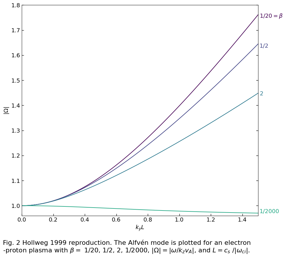
Note
Hollweg takes \(k_{\perp}=k_{y}\) for k propagating in the \(y\)-\(z\) plane as in the plot above. Contrarily, Bellan takes \(k_{\perp}=k_{x}\) for k propagating in the \(x\)-\(z\) plane.