This page was generated by nbsphinx from docs/notebooks/formulary/ExB_drift.ipynb.
Interactive online version: .

%matplotlib inline

import math

import astropy.units as u
import matplotlib.pyplot as plt
import numpy as np

from plasmapy import formulary, particles

Physics of the E×B drift

Consider a single particle of mass \(m\) and charge \(q\) in a constant, uniform magnetic field \(\mathbf{B}=B\ \hat{\mathbf{z}}\). In the absence of external forces, it travels with velocity \(\mathbf{v}\) governed by the equation of motion

\[m\frac{d\mathbf{v}}{dt} = q\mathbf{v}\times\mathbf{B}\]

which equates the net force on the particle to the corresponding Lorentz force. Assuming the particle initially (at time \(t=0\)) has \(\mathbf{v}\) in the \(x,z\) plane (with \(v_y=0\)), solving reveals

\[v_x = v_\perp\cos\omega_c t \quad\mathrm{;}\quad v_y = -\frac{q}{\lvert q \rvert}v_\perp\sin \omega_c t\]

while the parallel velocity \(v_z\) is constant. This indicates that the particle gyrates in a circular orbit in the \(x,y\) plane with constant speed \(v_\perp\), angular frequency \(\omega_c = \frac{\lvert q\rvert B}{m}\), and Larmor radius \(r_L=\frac{v_\perp}{\omega_c}\).

As an example, take one proton p+ moving with velocity \(1\ m/s\) in the \(x\)-direction at \(t=0\):

# Initialize proton in uniform B field
B = 5 * u.T
proton = particles.Particle("p+")
omega_c = formulary.frequencies.gyrofrequency(B, proton)
v_perp = 1 * u.m / u.s
r_L = formulary.lengths.gyroradius(B, proton, Vperp=v_perp)

We can define a function that evolves the particle’s position according to the relations above describing \(v_x,v_y\), and \(v_z\). The option to add a constant drift velocity \(v_d\) to the solution is included as an argument, though this drift velocity is zero by default:

def single_particle_trajectory(v_d=np.array([0, 0, 0])):
    # Set time resolution & velocity such that proton goes 1 meter along B per rotation
    T = 2 * math.pi / omega_c.value  # rotation period
    v_parallel = 1 / T * u.m / u.s
    dt = T / 1e2 * u.s

    # Set initial particle position
    x = []
    y = []
    xt = 0 * u.m
    yt = -r_L

    # Evolve motion
    timesteps = np.arange(0, 10 * T, dt.value)
    for t in list(timesteps):
        v_x = v_perp * math.cos(omega_c.value * t) + v_d[0]
        v_y = v_perp * math.sin(omega_c.value * t) + v_d[1]
        xt += +v_x * dt
        yt += +v_y * dt
        x.append(xt.value)
        y.append(yt.value)
    x = np.array(x)
    y = np.array(y)
    z = v_parallel.value * timesteps

    return x, y, z

Executing with the default argument and plotting the particle trajectory gives the expected helical motion, with a radius equal to the Larmor radius:

x, y, z = single_particle_trajectory()

fig = plt.figure(figsize=(6, 6))
ax = fig.add_subplot(111, projection="3d")
ax.plot(x, y, z, label=r"$\mathbf{F}=0$")
ax.legend()
bound = 3 * r_L.value
ax.set_xlim([-bound, bound])
ax.set_ylim([-bound, bound])
ax.set_zlim([0, 10])
ax.set_xlabel("x [m]")
ax.set_ylabel("y [m]")
ax.set_zlabel("z [m]")
plt.show()

print(f"r_L = {r_L.value:.2e} m")
print(f"omega_c = {omega_c.value:.2e} rads/s")

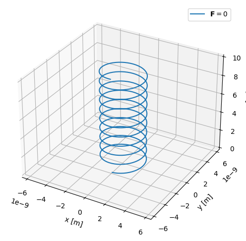
r_L = 2.09e-09 m
omega_c = 4.79e+08 rads/s

How does this motion change when a constant external force \(\mathbf{F}\) is added? The new equation of motion is

\[m\frac{d\mathbf{v}}{dt} = q\mathbf{v}\times\mathbf{B} + \mathbf{F}\]

and we can find a solution by considering velocities of the form \(\mathbf{v}=\mathbf{v}_\parallel + \mathbf{v}_L + \mathbf{v}_d\). Here, \(\mathbf{v}_\parallel\) is the velocity parallel to the magnetic field, \(\mathbf{v}_L\) is the Larmor gyration velocity in the absence of \(\mathbf{F}\) found previously, and \(\mathbf{v}_d\) is some constant drift velocity perpendicular to the magnetic field. Then, we find that

\[F_\parallel = m\frac{dv_\parallel}{dt} \quad\mathrm{and}\quad \mathbf{F}_\perp = q\mathbf{B}\times \mathbf{v}_d\]

and applying the vector triple product yields

\[\mathbf{v}_d = \frac{1}{q}\frac{\mathbf{F}_\perp\times\mathbf{B}}{B^2}\]

In the case where the external force \(\mathbf{F} = q\mathbf{E}\) is due to a constant electric field, this is the constant \(\mathbf{E}\times\mathbf{B}\) drift velocity:

\[\boxed{ \mathbf{v}_d = \frac{\mathbf{E}\times\mathbf{B}}{B^2} }\]

Built in drift functions allow you to account for the new force added to the system in two different ways:

E = 0.2 * u.V / u.m  # E-field magnitude
ey = np.array([0, 1, 0])
ez = np.array([0, 0, 1])
F = proton.charge * E  # force due to E-field

v_d = formulary.drifts.force_drift(F * ey, B * ez, proton.charge)
print("F drift velocity: ", v_d)
v_d = formulary.drifts.ExB_drift(E * ey, B * ez)
print("ExB drift velocity: ", v_d)

F drift velocity:  [0.04 0.   0.  ] m / s
ExB drift velocity:  [0.04 0.   0.  ] m / s

The resulting particle trajectory can be compared to the case without drifts by calling our previously defined function with the drift velocity now as an argument. As expected, there is a constant drift in the direction of \(\mathbf{E}\times\mathbf{B}\):

x_d, y_d, z_d = single_particle_trajectory(v_d=v_d)

fig = plt.figure(figsize=(6, 6))
ax = fig.add_subplot(111, projection="3d")
ax.plot(x, y, z, label=r"$\mathbf{F}=0$")
ax.plot(x_d, y_d, z_d, label=r"$\mathbf{F}=q\mathbf{E}$")

bound = 3 * r_L.value
ax.set_xlim([-bound, bound])
ax.set_ylim([-bound, bound])
ax.set_zlim([0, 10])
ax.set_xlabel("x [m]")
ax.set_ylabel("y [m]")
ax.set_zlabel("z [m]")
ax.legend()
plt.show()

print(f"r_L = {r_L.value:.2e} m")
print(f"omega_c = {omega_c.value:.2e} rads/s")

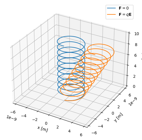
r_L = 2.09e-09 m
omega_c = 4.79e+08 rads/s

Of course, the implementation in our single_particle_trajectory() function requires the analytical solution for the velocity \(\mathbf{v}_d\). This solution can be compared with that implemented in the particle tracker notebook. It uses the Boris algorithm to evolve the particle along its trajectory in prescribed \(\mathbf{E}\) and \(\mathbf{B}\) fields, and thus does not require the analytical solution.