This page was generated by
nbsphinx from
docs/notebooks/diagnostics/charged_particle_radiography_particle_tracing_custom_source.ipynb.
Interactive online version:
![]() .
.
Synthetic Radiographs with Custom Source Profiles
In real charged particle radiography experiments, the finite size and distribution of the particle source limits the resolution of the radiograph. Some realistic sources produce particles with a non-uniform angular distribution that then superimposes a large scale “source profile” on the radiograph. For these reasons, the Tracker particle tracing class allows users to specify their own initial particle positions and velocities. This example will demonstrate how to use this functionality to create a more realistic synthetic radiograph that includes the effects from a non-uniform, finite source profile.
[1]:
import warnings

import astropy.units as u
import matplotlib.pyplot as plt
import numpy as np

from plasmapy.diagnostics.charged_particle_radiography import (
    synthetic_radiography as cpr,
)
from plasmapy.formulary.mathematics import rot_a_to_b
from plasmapy.particles import Particle
from plasmapy.plasma.grids import CartesianGrid
Contents
Creating Particles
In this example we will create a source of 1e5 protons with a 5% variance in energy, a non-uniform angular velocity distribution, and a finite size.
We will choose a setup in which the source-detector axis is parallel to the \(y\)-axis.
[3]:
# define location of source and detector plane
source = (0 * u.mm, -10 * u.mm, 0 * u.mm)
detector = (0 * u.mm, 100 * u.mm, 0 * u.mm)
Creating the Initial Particle Velocities
We will create the source distribution by utilizing the method of separation of variables,
and separately define the distribution component for each independent variable, \(u(v)\), \(g(\theta)\), and \(h(\phi)\). For geometric convenience, we will generate the velocity vector distribution around the \(z\)-axis and then rotate the final velocities to be parallel to the source-detector axis (in this case the \(y\)-axis).
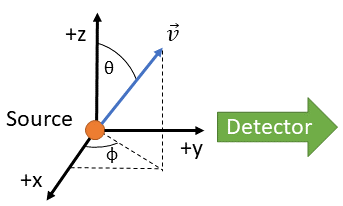
First we will create the orientation angles polar (\(\theta\)) and azimuthal (\(\phi\)) for each particle. Generating \(\phi\) is simple: we will choose the azimuthal angles to just be uniformly distributed
[4]:
phi = np.random.uniform(high=2 * np.pi, size=int(nparticles))
However, choosing \(\theta\) is more complicated. Since the solid angle \(d\Omega = sin \theta d\theta d\phi\), if we draw a uniform distribution of \(\theta\) we will create a non-uniform distribution of particles in solid angle. This will create a sharp central peak on the detector plane.
[5]:
theta = np.random.uniform(high=np.pi / 2, size=int(nparticles))

fig, ax = plt.subplots(figsize=(6, 6))
theta_per_sa, bins = np.histogram(theta, bins=100, weights=1 / np.sin(theta))
ax.set_xlabel("$\\theta$ (rad)", fontsize=14)
ax.set_ylabel("N/N$_0$ per  d$\\Omega$", fontsize=14)
ax.plot(bins[1:], theta_per_sa / np.sum(theta_per_sa))
ax.set_title(f"N$_0$ = {nparticles:.0e}", fontsize=14)
ax.set_yscale("log")
ax.set_xlim(0, np.pi / 2)
ax.set_ylim(None, 1);
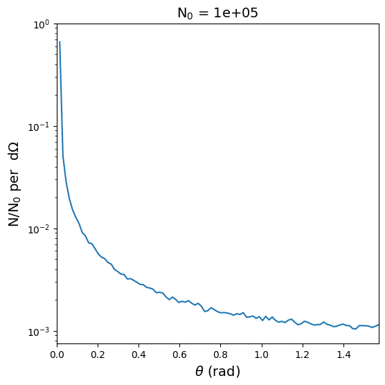
To create a uniform distribution in solid angle, we need to draw values of \(\theta\) with a probability distribution weighted by \(\sin \theta\). This can be done using the np.random.choice() function, which draws size elements from a distribution arg with a probability distribution prob. Setting the replace keyword allows the same arguments to be drawn multiple times.
[6]:
arg = np.linspace(0, np.pi / 2, num=int(1e5))
prob = np.sin(arg)
prob *= 1 / np.sum(prob)
theta = np.random.choice(arg, size=int(nparticles), replace=True, p=prob)

fig, ax = plt.subplots(figsize=(6, 6))
theta_per_sa, bins = np.histogram(theta, bins=100, weights=1 / np.sin(theta))
ax.plot(bins[1:], theta_per_sa / np.sum(theta_per_sa))
ax.set_xlabel("$\\theta$ (rad)", fontsize=14)
ax.set_ylabel("N/N$_0$ per  d$\\Omega$", fontsize=14)
ax.set_title(f"N$_0$ = {nparticles:.0e}", fontsize=14)
ax.set_yscale("log")
ax.set_xlim(0, np.pi / 2)
ax.set_ylim(None, 0.1);
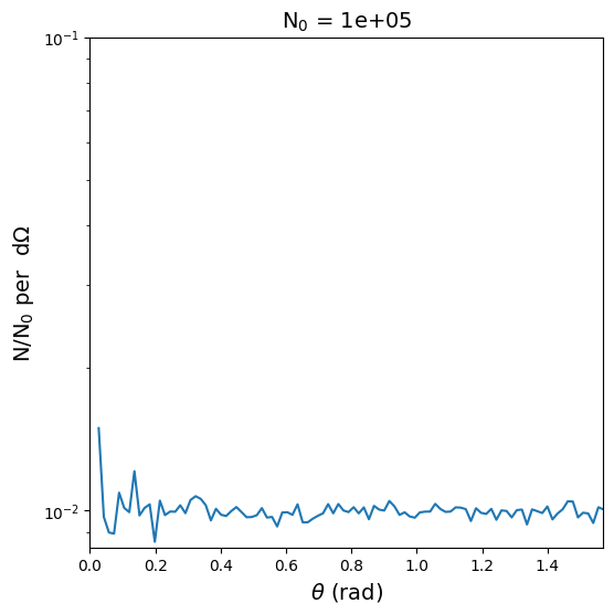
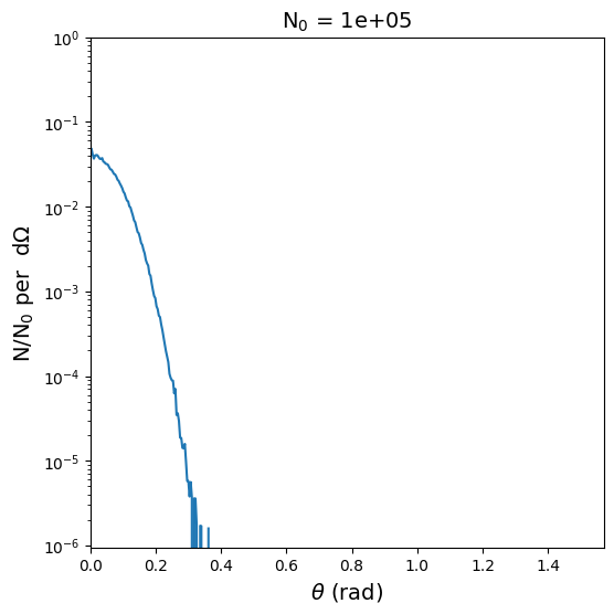
Now that we have a \(\theta\) distribution that is uniform in solid angle, we can perturb it by adding additional factors to the probability distribution used in np.random.choice(). For this case, let’s create a Gaussian distribution in solid angle.
Since particles moving at large angles will not be seen in the synthetic radiograph, we will set an upper bound \(\theta_{max}\) on the argument here. This is equivalent to setting the max_theta keyword in create_particles()
[7]:
arg = np.linspace(0, np.pi / 8, num=int(1e5))
prob = np.sin(arg) * np.exp(-(arg**2) / 0.1**2)
prob *= 1 / np.sum(prob)
theta = np.random.choice(arg, size=int(nparticles), replace=True, p=prob)

fig, ax = plt.subplots(figsize=(6, 6))
theta_per_sa, bins = np.histogram(theta, bins=100, weights=1 / np.sin(theta))
ax.plot(bins[1:], theta_per_sa / np.sum(theta_per_sa))
ax.set_title(f"N$_0$ = {nparticles:.0e}", fontsize=14)
ax.set_xlabel("$\\theta$ (rad)", fontsize=14)
ax.set_ylabel("N/N$_0$ per  d$\\Omega$", fontsize=14)
ax.set_yscale("log")
ax.set_xlim(0, np.pi / 2)
ax.set_ylim(None, 1);
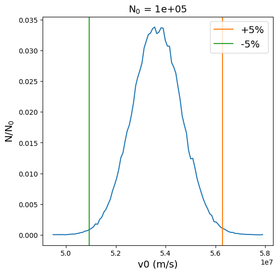
Now that the angular distributions are done, we will determine the energy (speed) for each particle. For this example, we will assume that the particle energy distribution is not a function of angle. We will create a Gaussian distribution of speeds with ~5% variance centered on a particle energy of 15 MeV.
[8]:
v_cent = np.sqrt(2 * 15 * u.MeV / particle.mass).to(u.m / u.s).value
v0 = np.random.normal(loc=v_cent, scale=1e6, size=int(nparticles))
v0 *= u.m / u.s

fig, ax = plt.subplots(figsize=(6, 6))
v_per_bin, bins = np.histogram(v0.si.value, bins=100)
ax.plot(bins[1:], v_per_bin / np.sum(v_per_bin))
ax.set_title(f"N$_0$ = {nparticles:.0e}", fontsize=14)
ax.set_xlabel("v0 (m/s)", fontsize=14)
ax.set_ylabel("N/N$_0$", fontsize=14)
ax.axvline(x=1.05 * v_cent, label="+5%", color="C1")
ax.axvline(x=0.95 * v_cent, label="-5%", color="C2")
ax.legend(fontsize=14, loc="upper right");
Next, we will construct velocity vectors centered around the z-axis for each particle.
[9]:
Finally, we will use the function rot_a_to_b() to create a rotation matrix that will rotate the vel distribution so the distribution is centered about the \(y\) axis instead of the \(z\) axis.
Since the velocity vector distribution should be symmetric about the \(y\) axis, we can confirm this by checking that the normalized average velocity vector is close to the \(y\) unit vector.
[11]:
avg_v = np.mean(vel, axis=0)
print(avg_v / np.linalg.norm(avg_v))
[-1.56950008e-04 9.99999983e-01 9.68603269e-05]
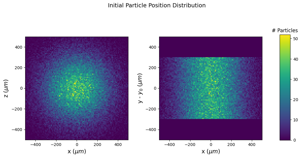
Creating the Initial Particle Positions
For this example, we will create an initial position distribution representing a laser spot centered on the source location defined above as source. The distribution will be cylindrical (oriented along the \(y\)-axis) with a uniform distribution in y and a Gaussian distribution in radius (in the xz plane). We therefore need to create distributions in \(y\), \(\theta\), and \(r\), and then transform those into Cartesian positions.
Just as we previously weighted the \(\theta\) distribution with a \(sin \theta\) probability distribution to generate a uniform distribution in solid angle, we need to weight the \(r\) distribution with a \(r\) probability distribution so that the particles are uniformly distributed over the area of the disk.
[12]:
dy = 300 * u.um
y = np.random.uniform(
    low=(source[1] - dy).to(u.m).value,
    high=(source[1] + dy).to(u.m).value,
    size=int(nparticles),
)

arg = np.linspace(1e-9, 1e-3, num=int(1e5))
prob = arg * np.exp(-((arg / 3e-4) ** 2))
prob *= 1 / np.sum(prob)
r = np.random.choice(arg, size=int(nparticles), replace=True, p=prob)


theta = np.random.uniform(low=0, high=2 * np.pi, size=int(nparticles))

x = r * np.cos(theta)
z = r * np.sin(theta)

hist, xpos, zpos = np.histogram2d(
    x * 1e6,
    z * 1e6,
    bins=[100, 100],
    range=np.array([[-5e2, 5e2], [-5e2, 5e2]]),
)

hist2, xpos2, ypos = np.histogram2d(
    x * 1e6,
    (y - source[1].to(u.m).value) * 1e6,
    bins=[100, 100],
    range=np.array([[-5e2, 5e2], [-5e2, 5e2]]),
)

fig, ax = plt.subplots(ncols=2, figsize=(12, 6))
fig.subplots_adjust(wspace=0.3, right=0.8)
fig.suptitle("Initial Particle Position Distribution", fontsize=14)
vmax = np.max([np.max(hist), np.max(hist2)])

p1 = ax[0].pcolormesh(xpos, zpos, hist.T, vmax=vmax)
ax[0].set_xlabel("x ($\\mu m$)", fontsize=14)
ax[0].set_ylabel("z ($\\mu m$)", fontsize=14)
ax[0].set_aspect("equal")

p2 = ax[1].pcolormesh(xpos2, ypos, hist2.T, vmax=vmax)
ax[1].set_xlabel("x ($\\mu m$)", fontsize=14)
ax[1].set_ylabel("y - $y_0$ ($\\mu m$)", fontsize=14)
ax[1].set_aspect("equal")

cbar_ax = fig.add_axes([0.85, 0.2, 0.03, 0.6])
cbar_ax.set_title("# Particles")
fig.colorbar(p2, cax=cbar_ax);
Finally we will combine these position arrays into an array with units.
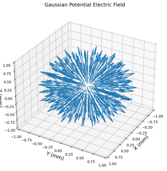
Creating a Synthetic Radiograph
To create an example synthetic radiograph, we will first create a field grid representing the analytical electric field produced by a sphere of Gaussian potential.
[14]:
# Create a Cartesian grid
L = 1 * u.mm
grid = CartesianGrid(-L, L, num=100)

# Create a spherical potential with a Gaussian radial distribution
radius = np.linalg.norm(grid.grid, axis=3)
arg = (radius / (L / 3)).to(u.dimensionless_unscaled)
potential = 6e5 * np.exp(-(arg**2)) * u.V

# Calculate E from the potential
Ex, Ey, Ez = np.gradient(potential, grid.dax0, grid.dax1, grid.dax2)
mask = radius < L / 2
Ex = -np.where(mask, Ex, 0)
Ey = -np.where(mask, Ey, 0)
Ez = -np.where(mask, Ez, 0)

# Add those quantities to the grid
grid.add_quantities(E_x=Ex, E_y=Ey, E_z=Ez, phi=potential)


# Plot the E-field
fig = plt.figure(figsize=(8, 8))
ax = fig.add_subplot(111, projection="3d")
ax.view_init(30, 30)

# skip some points to make the vector plot intelligible
s = tuple([slice(None, None, 6)] * 3)

ax.quiver(
    grid.pts0[s].to(u.mm).value,
    grid.pts1[s].to(u.mm).value,
    grid.pts2[s].to(u.mm).value,
    grid["E_x"][s],
    grid["E_y"][s],
    grid["E_z"][s],
    length=5e-7,
)

ax.set_xlabel("X (mm)", fontsize=14)
ax.set_ylabel("Y (mm)", fontsize=14)
ax.set_zlabel("Z (mm)", fontsize=14)
ax.set_xlim(-1, 1)
ax.set_ylim(-1, 1)
ax.set_zlim(-1, 1)
ax.set_title("Gaussian Potential Electric Field", fontsize=14);
We will then create the synthetic radiograph object. The warning filter ignores a warning that arises because \(B_x\), \(B_y\), \(B_z\) are not provided in the grid (they will be assumed to be zero).
[15]:
with warnings.catch_warnings():
    warnings.simplefilter("ignore")
    sim = cpr.Tracker(grid, source, detector, verbose=False)
Now, instead of using create_particles() to create the particle distribution, we will use the load_particles() function to use the particles we have created above.
[16]:
sim.load_particles(pos, vel, particle=particle)
Now the particle radiograph simulation can be run as usual.
[17]:
sim.run();
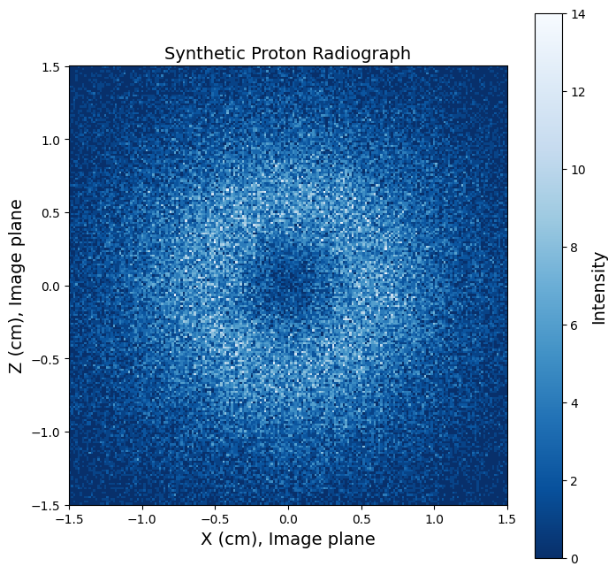
[18]:
size = np.array([[-1, 1], [-1, 1]]) * 1.5 * u.cm
bins = [200, 200]
hax, vax, intensity = cpr.synthetic_radiograph(sim, size=size, bins=bins)

fig, ax = plt.subplots(figsize=(8, 8))
plot = ax.pcolormesh(
    hax.to(u.cm).value,
    vax.to(u.cm).value,
    intensity.T,
    cmap="Blues_r",
    shading="auto",
)
cb = fig.colorbar(plot)
cb.ax.set_ylabel("Intensity", fontsize=14)
ax.set_aspect("equal")
ax.set_xlabel("X (cm), Image plane", fontsize=14)
ax.set_ylabel("Z (cm), Image plane", fontsize=14)
ax.set_title("Synthetic Proton Radiograph", fontsize=14);
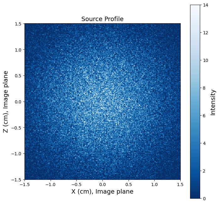
Calling the synthetic_radiograph() function with the ignore_grid keyword will produce the synthetic radiograph corresponding to the source profile propagated freely through space (i.e. in the absence of any grid fields).
[19]:
hax, vax, intensity = cpr.synthetic_radiograph(
    sim,
    size=size,
    bins=bins,
    ignore_grid=True,
)

fig, ax = plt.subplots(figsize=(8, 8))
plot = ax.pcolormesh(
    hax.to(u.cm).value,
    vax.to(u.cm).value,
    intensity.T,
    cmap="Blues_r",
    shading="auto",
)
cb = fig.colorbar(plot)
cb.ax.set_ylabel("Intensity", fontsize=14)
ax.set_aspect("equal")
ax.set_xlabel("X (cm), Image plane", fontsize=14)
ax.set_ylabel("Z (cm), Image plane", fontsize=14)
ax.set_title("Source Profile", fontsize=14);
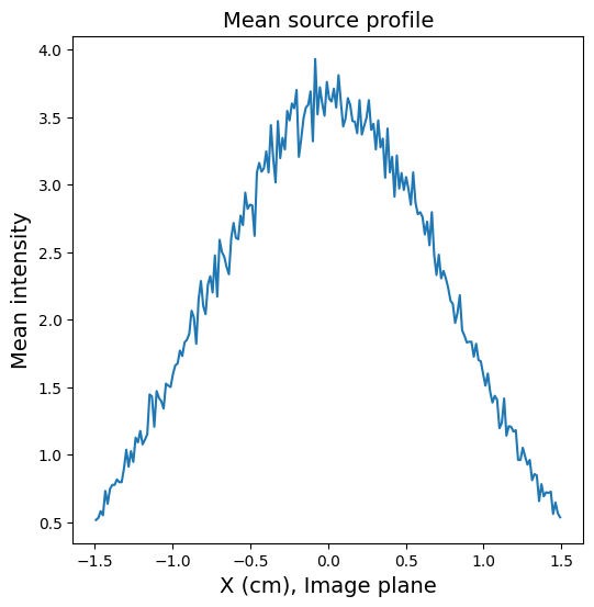
[20]:
fig, ax = plt.subplots(figsize=(6, 6))
ax.plot(hax.to(u.cm).value, np.mean(intensity, axis=0))
ax.set_xlabel("X (cm), Image plane", fontsize=14)
ax.set_ylabel("Mean intensity", fontsize=14)
ax.set_title("Mean source profile", fontsize=14);