This page was generated by nbsphinx from docs/notebooks/diagnostics/langmuir_analysis.ipynb.
Interactive online version: .

Langmuir probe data analysis

Let’s analyze a few Langmuir probe characteristics using the diagnostics.langmuir subpackage. First we need to import the module and some basics.

%matplotlib inline

from pathlib import Path
from pprint import pprint

import astropy.units as u
import numpy as np

from plasmapy.diagnostics.langmuir import Characteristic, swept_probe_analysis

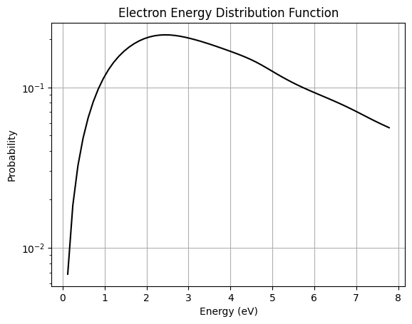
The first characteristic we analyze is a simple single-probe measurement in a low (ion) temperature, low density plasma with a cylindrical probe. This allows us to utilize OML theory implemented in swept_probe_analysis(). The data has been preprocessed with some smoothing, which allows us to obtain a Electron Energy Distribution Function (EEDF) as well.

# Load the bias and current values stored in the .p pickle file.
path = (Path.cwd() / ".." / "langmuir_samples" / "Beckers2017.npy").resolve()
bias, current = np.load(path)

# Create the Characteristic object, taking into account the correct units
characteristic = Characteristic(u.Quantity(bias, u.V), u.Quantity(current, u.A))

# Calculate the cylindrical probe surface area
probe_length = 1.145 * u.mm
probe_diameter = 1.57 * u.mm
probe_area = probe_length * np.pi * probe_diameter + np.pi * 0.25 * probe_diameter**2

/home/docs/checkouts/readthedocs.org/user_builds/plasmapy/envs/latest/lib/python3.12/site-packages/plasmapy/diagnostics/langmuir.py:36: FutureWarning: The plasmapy.diagnostics.langmuir module will be deprecated in favor of the plasmapy.analysis.swept_langmuir sub-package and phased out over 2021.  The plasmapy.analysis package was released in v0.5.0.
  warnings.warn(

Now we can actually perform the analysis. Since the plasma is in Helium an ion mass number of 4 is entered. The results are visualized and the obtained EEDF is also shown.

pprint(
    swept_probe_analysis(
        characteristic, probe_area, "He-4+", visualize=True, plot_EEDF=True
    )
)

{'I_es': <Quantity 0.01873572 A>,
 'I_is': <Quantity -0.00231536 A>,
 'T_e': <Quantity 2.41021849 eV>,
 'V_F': <Quantity -5.75541887 V>,
 'V_P': <Quantity 2.15098227 V>,
 'n_e': <Quantity 5.93671704e+16 1 / m3>,
 'n_i': <Quantity 4.1665378e+17 1 / m3>,
 'n_i_OML': <Quantity 1.69390014e+17 1 / m3>}

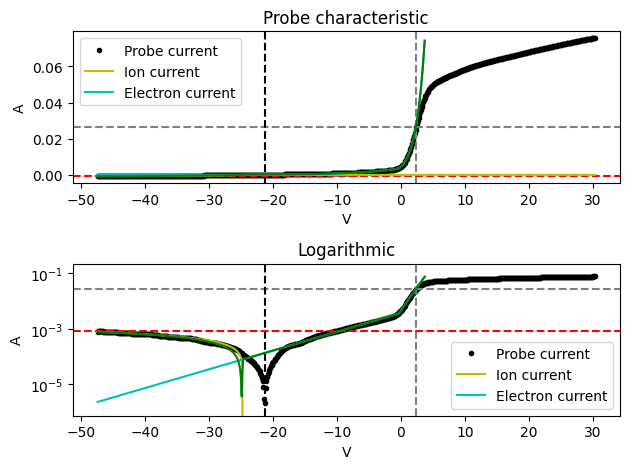
The cyan and yellow lines indicate the fitted electron and ion currents, respectively. The green line is the sum of these and agrees nicely with the data. This indicates a successful analysis.

The next sample probe data is provided by David Pace. It is also obtained from a low relatively ion temperature and density plasma, in Argon.

# Load the data from a file and create the Characteristic object
path = (Path.cwd() / ".." / "langmuir_samples" / "Pace2015.npy").resolve()
bias, current = np.load(path)
characteristic = Characteristic(u.Quantity(bias, u.V), u.Quantity(current, u.A))

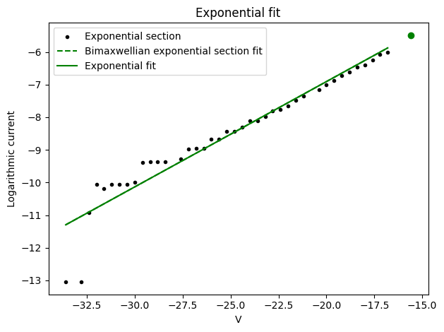
Initially the electrons are assumed to be Maxwellian. To check this the fit of the electron growth region will be plotted.

swept_probe_analysis(
    characteristic,
    0.738 * u.cm**2,
    "Ar-40 1+",
    bimaxwellian=False,
    plot_electron_fit=True,
)

{'V_P': <Quantity -16.4 V>,
 'V_F': <Quantity -35.6 V>,
 'I_es': <Quantity 0.00282382 A>,
 'I_is': <Quantity -0.000129 A>,
 'n_e': <Quantity 7.60824393e+14 1 / m3>,
 'n_i': <Quantity 6.23732194e+15 1 / m3>,
 'T_e': <Quantity 3.51990716 eV>,
 'n_i_OML': <Quantity 3.07522416e+15 1 / m3>}

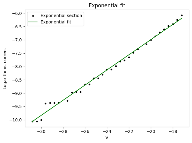
It can be seen that this plasma is slightly bi-Maxwellian, as there are two distinct slopes in the exponential section. The analysis is now performed with bimaxwellian set to True, which yields improved results.

pprint(
    swept_probe_analysis(
        characteristic,
        0.738 * u.cm**2,
        "Ar-40 1+",
        bimaxwellian=True,
        visualize=True,
        plot_electron_fit=True,
    )
)

/home/docs/checkouts/readthedocs.org/user_builds/plasmapy/envs/latest/lib/python3.12/site-packages/plasmapy/diagnostics/langmuir.py:1075: RuntimeWarning: overflow encountered in exp
  np.exp(fit_func(probe_characteristic.bias.to(u.V).value, *fit)) * u.A

{'I_es': <Quantity 0.00282382 A>,
 'I_is': <Quantity -0.000129 A>,
 'T_e': <Quantity [1.77947044e-07, 3.09914301e+00] eV>,
 'V_F': <Quantity -35.6 V>,
 'V_P': <Quantity -16.4 V>,
 'hot_fraction': 1.0,
 'n_e': <Quantity 8.10828907e+14 1 / m3>,
 'n_i': <Quantity 6.64726444e+15 1 / m3>,
 'n_i_OML': <Quantity 3.07522416e+15 1 / m3>}

The probe current resolution of the raw data is relatively poor, but the analysis still performs well in the ion current region. The bi-Maxwellian properties are not significant but do make a difference. Check this analysis without setting bimaxwellian to True! This is reflected in the results, which indicate that the temperatures of the cold and hot electron population are indeed different, but relatively close.

This Helium plasma is fully bi-Maxwellian.

# Import probe data and calculate probe surface area.
path = (Path.cwd() / ".." / "langmuir_samples" / "Beckers2017b.npy").resolve()
bias, current = np.load(path)
characteristic = Characteristic(u.Quantity(bias, u.V), u.Quantity(current, u.A))
probe_length = 1.145 * u.mm
probe_diameter = 1.57 * u.mm
probe_area = probe_length * np.pi * probe_diameter + np.pi * 0.25 * probe_diameter**2

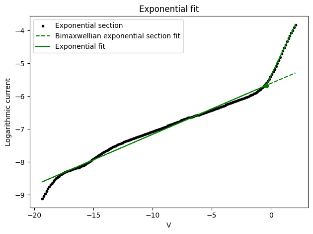
plot_electron_fit is set to True to check the bi-Maxwellian properties. The fit converges nicely to the two slopes of the electron growth region.

pprint(
    swept_probe_analysis(
        characteristic,
        probe_area,
        "He-4+",
        bimaxwellian=True,
        plot_electron_fit=True,
        visualize=True,
    )
)

{'I_es': <Quantity 0.02655063 A>,
 'I_is': <Quantity -0.00080287 A>,
 'T_e': <Quantity [1.33644199, 6.45311087] eV>,
 'V_F': <Quantity -21.29773863 V>,
 'V_P': <Quantity 2.42370446 V>,
 'hot_fraction': 0.188060045293475,
 'n_e': <Quantity 8.6146857e+16 1 / m3>,
 'n_i': <Quantity 1.47942378e+17 1 / m3>,
 'n_i_OML': <Quantity 6.08613986e+16 1 / m3>}