This page was generated by nbsphinx from docs/notebooks/diagnostics/charged_particle_radiography_film_stacks.ipynb.
Interactive online version: .

Synthetic Charged Particle Radiographs with Multiple Detector Layers

Charged particle radiographs are often recorded on detector stacks with multiple layers (often either radiochromic film or CR39 plastic). Since charged particles deposit most of their energy at a depth related to their energy (the Bragg peak), each detector layer records a different energy band of particles. The energy bands recorded on each layer are further discriminated by including layers of filter material (eg. thin strips of aluminum) between the active layers. In order to analyze this data, it is necessary to calculate what range of particle energies are stopped in each detector layer.

The charged_particle_radiography module includes a tool for calculating the energy bands for a given stack of detectors. This calculation is a simple approximation (more accurate calculations can be made using Monte Carlo codes), but is sufficient in many cases.

from tempfile import gettempdir

import astropy.units as u
import matplotlib.pyplot as plt
import numpy as np

from plasmapy.diagnostics.charged_particle_radiography.detector_stacks import (
    Layer,
    Stack,
)
from plasmapy.utils.data.downloader import Downloader

The charged_particle_radiography module represents a detector stack with a Stack object, which contains an ordered list of Layer objects. In this example, we will create a list of Layer objects, use them to initialize a Stack, then compute the energy bands.

Each Layer is defined by the following required properties: - thickness: an astropy Quantity defining the thickness of the layer. - active: a boolean flag which indicates whether the layer is active (detector) or inactive (eg. a filter). - energy_axis: An astropy Quantity array of energies. - stopping_power: An astropy Quantity array containing the product of stopping power and material density at each energy in energy_axis.

The stopping power in various materials for protons and electrons is tabulated by NIST in the PSTAR and ESTAR databases. The stopping powers are tabulated in units of MeV cm\(^2\) / g, so the product of stopping power and density has units of MeV/cm.

For this demonstration, we will load two stopping power tables, downloaded from PSTAR, for aluminum and a human tissue equivalent that is a good approximation for many radiochromic films.

temp_dir = gettempdir()  # Get a temporary directory to save the files
dl = Downloader(directory=temp_dir, validate=False)
tissue_path = dl.get_file("NIST_PSTAR_tissue_equivalent.txt")
aluminum_path = dl.get_file("NIST_PSTAR_aluminum.txt")

These files can be directly downloaded from PSTAR, and the contents look like this

with open(tissue_path) as f:
    for i in range(15):
        print(f.readline(), end="")
print("...")

PSTAR: Stopping Powers and Range Tables for Protons

A-150 TISSUE-EQUIVALENT PLASTIC

Kinetic   Total
Energy    Stp. Pow.
MeV       MeV cm2/g

1.000E-03 2.215E+02
1.500E-03 2.523E+02
2.000E-03 2.803E+02
2.500E-03 3.059E+02
3.000E-03 3.297E+02
4.000E-03 3.705E+02
5.000E-03 4.075E+02
...

Now we will load the energy and stopping power arrays from the files.

arr = np.loadtxt(tissue_path, skiprows=8)
energy_axis = arr[:, 0] * u.MeV
tissue_density = 1.04 * u.g / u.cm**3
tissue_stopping_power = arr[:, 1] * u.MeV * u.cm**2 / u.g * tissue_density

arr = np.loadtxt(aluminum_path, skiprows=8)
aluminum_density = 2.7 * u.g / u.cm**3
aluminum_stopping_power = arr[:, 1] * u.MeV * u.cm**2 / u.g * aluminum_density

If we plot the stopping powers as a function of energy on a log-log scale, we see that they are non-linear, with much higher values at lower energies. This is why particles deposit most of their energy at a characteristic depth. As particles propagate into material, they lose energy slowly at first. But, as they loose energy, the effective stopping power increases expontentially.

fig, ax = plt.subplots()
ax.plot(energy_axis.value, tissue_stopping_power, label="Tissue equivalent")
ax.plot(energy_axis.value, aluminum_stopping_power, label="Aluminum")
ax.set_xscale("log")
ax.set_yscale("log")
ax.set_xlabel("Energy (MeV)")
ax.set_ylabel("Stopping power (MeV/cm)")
ax.legend();

Before creating a Stack, we will start by creating a list that represents a common type of radiochromic film, HD-V2. HD-V2 consists of two layers: a 12 \(\mu\)m active layer deposited on a 97 \(\mu\)m substrate. The stopping powers of both layers are similar to human tissue (by design, HD-V2 is commonly used for medical research).

HDV2 = [
    Layer(12 * u.um, energy_axis, tissue_stopping_power, active=True),
    Layer(97 * u.um, energy_axis, tissue_stopping_power, active=False),
]

We will now create a list of layers of HDV2 separated by aluminum filter layers of various thickness, then use this list to instantiate a Stack object

layers = [
    Layer(100 * u.um, energy_axis, aluminum_stopping_power, active=False),
    *HDV2,
    Layer(100 * u.um, energy_axis, aluminum_stopping_power, active=False),
    *HDV2,
    Layer(100 * u.um, energy_axis, aluminum_stopping_power, active=False),
    *HDV2,
    Layer(100 * u.um, energy_axis, aluminum_stopping_power, active=False),
    *HDV2,
    Layer(500 * u.um, energy_axis, aluminum_stopping_power, active=False),
    *HDV2,
    Layer(500 * u.um, energy_axis, aluminum_stopping_power, active=False),
    *HDV2,
    Layer(1000 * u.um, energy_axis, aluminum_stopping_power, active=False),
    *HDV2,
    Layer(1000 * u.um, energy_axis, aluminum_stopping_power, active=False),
    *HDV2,
    Layer(2000 * u.um, energy_axis, aluminum_stopping_power, active=False),
    *HDV2,
    Layer(2000 * u.um, energy_axis, aluminum_stopping_power, active=False),
    *HDV2,
    Layer(2000 * u.um, energy_axis, aluminum_stopping_power, active=False),
]

stack = Stack(layers)

The number of layers, active layers, and the total thickness of the film stack are available as properties.

print(f"Number of layers: {stack.num_layers}")
print(f"Number of active layers: {stack.num_active}")
print(f"Total stack thickness: {stack.thickness:.2f}")

Number of layers: 31
Number of active layers: 10
Total stack thickness: 0.01 m

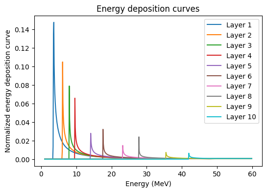
The curves of deposited energy per layer for a given array of energies can then be calculated using the deposition_curves() method. The stopping power for a particle can change significantly within a layer, so the stopping power is numerically integrated within each layer. The spatial resolution of this integration can be set using the dx keyword. Setting the return_only_active keyword means that deposition curves will only be returned for the active layers (inactive layers are still included in the calculation).

energies = np.arange(1, 60, 0.1) * u.MeV
deposition_curves = stack.deposition_curves(
    energies, dx=1 * u.um, return_only_active=True
);

fig, ax = plt.subplots(figsize=(6, 4))
ax.set_title("Energy deposition curves")
ax.set_xlabel("Energy (MeV)")
ax.set_ylabel("Normalized energy deposition curve")
for layer in range(stack.num_active):
    ax.plot(energies, deposition_curves[layer, :], label=f"Layer {layer+1}")
ax.legend();

We can look at the deposition curves including all layers (active and inactive) to see where particles of a given energy are deposited.

deposition_curves_all = stack.deposition_curves(energies, return_only_active=False)

fig, ax = plt.subplots(figsize=(6, 4))
ax.set_title("10 MeV Particles per layer")
ax.set_xlabel("Layer #")
ax.set_ylabel("Fraction of particles")
E0 = np.argmin(np.abs(10 * u.MeV - energies))
ax.plot(np.arange(stack.num_layers) + 1, deposition_curves_all[:, E0]);

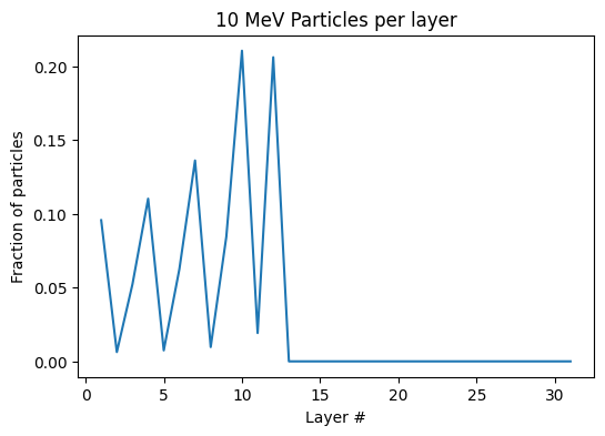
The sharp peaks correspond to the aluminum filter layers, which stop more particles than the film layers.

The deposition curve is normalized such that each value represents the fraction of particles with a given energy that will be stopped in that layer. Since all particles are stopped before the last layer, the sum over all layers (including the inactive layers) for a given energy is always unity.

integral = np.sum(deposition_curves_all, axis=0)
print(np.allclose(integral, 1))

True

We can quantify the range of initial particle energies primarily recorded on each film layer by calculating the full with at half maximum (FWHM) of the deposition curve for that layer. This calculation is done by the energy_bands() method, which returns an array of the \(\pm\) FWHM values for each film layer.

ebands = stack.energy_bands([0.1, 60] * u.MeV, 0.1 * u.MeV, return_only_active=True)
for layer in range(stack.num_active):
    print(
        f"Layer {layer+1}: {ebands[layer,0].value:.1f}-{ebands[layer,1].value:.1f} MeV"
    )

Layer 1: 0.0-0.0 MeV
Layer 2: 0.0-0.0 MeV
Layer 3: 0.0-0.0 MeV
Layer 4: 0.0-0.0 MeV
Layer 5: 0.0-0.0 MeV
Layer 6: 0.0-0.0 MeV
Layer 7: 0.0-0.0 MeV
Layer 8: 0.0-0.0 MeV
Layer 9: 0.0-0.0 MeV
Layer 10: 0.0-0.0 MeV

From this information, we can conclude see that the radiograph recorded on Layer 5 is primarily created by protons bwetween 12.5 and 12.8 MeV. This energy information can then be used to inform analysis of the images.