This page was generated by nbsphinx from docs/notebooks/analysis/fit_functions.ipynb.
Interactive online version: .

Fit Functions

Fit functions are a set of callable classes designed to aid in fitting analytical functions to data. A fit function class combines the following functionality:

1. An analytical function that is callable with given parameters or fitted parameters.

2. Curve fitting functionality (usually SciPy’s curve_fit() or linregress()), which stores the fit statistics and parameters into the class. This makes the function easily callable with the fitted parameters.

3. Error propagation calculations.

4. A root solver that returns either the known analytical solutions or uses SciPy’s fsolve() to calculate the roots.

%matplotlib inline

import matplotlib.pyplot as plt
import numpy as np

from plasmapy.analysis import fit_functions as ffuncs

plt.rcParams["figure.figsize"] = [10.5, 0.56 * 10.5]

Contents:

1. Fit function basics

2. Fitting to data

   1. Getting fit results

   2. Fit function is callable

   3. Plotting results

   4. Root solving

Fit function basics

There is an ever expanding collection of fit functions, but this notebook will use ExponentialPlusLinear as an example.

A fit function class has no required arguments at time of instantiation.

# basic instantiation
explin = ffuncs.ExponentialPlusLinear()

# fit parameters are not set yet
(explin.params, explin.param_errors)

(None, None)

Each fit parameter is given a name.

explin.param_names

('a', 'alpha', 'm', 'b')

These names are used throughout the fit function’s documentation, as well as in its __repr__, __str__, and latex_str methods.

(explin, explin.__str__(), explin.latex_str)

(f(x) = a exp(alpha x) + m x + b <class 'plasmapy.analysis.fit_functions.ExponentialPlusLinear'>,
 'f(x) = a exp(alpha x) + m x + b',
 'a \\, \\exp(\\alpha x) + m x + b')

Fitting to data

Fit functions provide the curve_fit() method to fit the analytical function to a set of \((x, y)\) data. This is typically done with SciPy’s curve_fit() function, but fitting is done with SciPy’s linregress() for the Linear fit function.

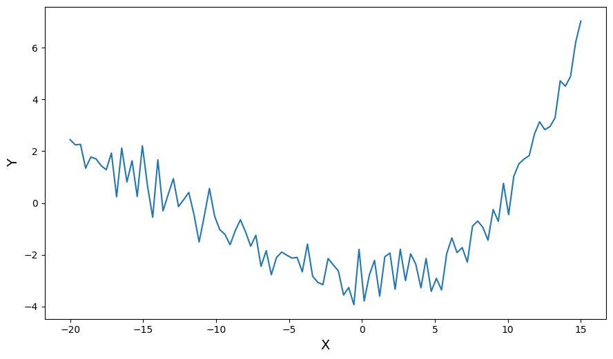
Let’s generate some noisy data to fit to…

params = (5.0, 0.1, -0.5, -8.0)  # (a, alpha, m, b)
xdata = np.linspace(-20, 15, num=100)
ydata = explin.func(xdata, *params) + np.random.normal(0.0, 0.6, xdata.size)

plt.plot(xdata, ydata)
plt.xlabel("X", fontsize=14)
plt.ylabel("Y", fontsize=14)

Text(0, 0.5, 'Y')

The fit function curve_fit() shares the same signature as SciPy’s curve_fit(), so any **kwargs will be passed on. By default, only the \((x, y)\) values are needed.

explin.curve_fit(xdata, ydata)

Getting fit results

After fitting, the fitted parameters, uncertainties, and coefficient of determination, or \(r^2\), values can be retrieved through their respective properties, params, parame_errors, and rsq.

(explin.params, explin.params.a, explin.params.alpha)

(FitParamTuple(a=4.5059236130548035, alpha=0.10680679831282214, m=-0.4801040605961944, b=-7.531630662967621),
 4.5059236130548035,
 0.10680679831282214)

(explin.param_errors, explin.param_errors.a, explin.param_errors.alpha)

(FitParamTuple(a=0.7882423166077, alpha=0.00806850478515761, m=0.037763589423132085, b=0.8135260377913293),
 0.7882423166077,
 0.00806850478515761)

explin.rsq

np.float64(0.9606654828748814)

Fit function is callable

Now that parameters are set, the fit function is callable.

explin(0)

np.float64(-3.0257070499128176)

Associated errors can also be generated.

y, y_err = explin(np.linspace(-1, 1, num=10), reterr=True)
(y, y_err)

(array([-3.00205627, -3.01148281, -3.01857322, -3.02327137, -3.02551981,
        -3.02525969, -3.02243077, -3.01697135, -3.00881825, -2.99790676]),
 array([1.07987898, 1.09067895, 1.10200945, 1.1138864 , 1.12632618,
        1.13934558, 1.15296188, 1.1671928 , 1.18205655, 1.19757184]))

Known uncertainties in \(x\) can be specified too.

y, y_err = explin(np.linspace(-1, 1, num=10), reterr=True, x_err=0.1)
(y, y_err)

(array([-3.00205627, -3.01148281, -3.01857322, -3.02327137, -3.02551981,
        -3.02525969, -3.02243077, -3.01697135, -3.00881825, -2.99790676]),
 array([1.07988947, 1.0906853 , 1.10201265, 1.11388751, 1.12632627,
        1.13934579, 1.15296338, 1.1671968 , 1.18206431, 1.19758466]))

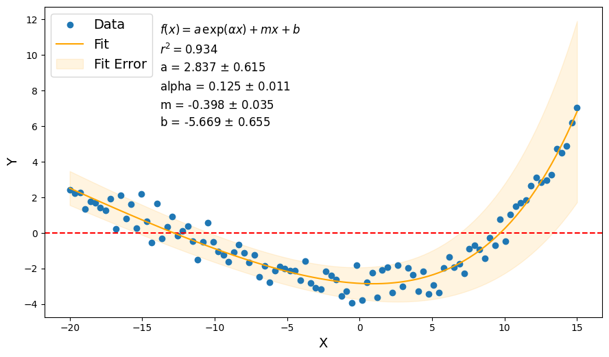
Plotting results

# plot original data
plt.plot(xdata, ydata, marker="o", linestyle=" ", label="Data")
ax = plt.gca()
ax.set_xlabel("X", fontsize=14)
ax.set_ylabel("Y", fontsize=14)

ax.axhline(0.0, color="r", linestyle="--")

# plot fitted curve + error
yfit, yfit_err = explin(xdata, reterr=True)
ax.plot(xdata, yfit, color="orange", label="Fit")
ax.fill_between(
    xdata,
    yfit + yfit_err,
    yfit - yfit_err,
    color="orange",
    alpha=0.12,
    zorder=0,
    label="Fit Error",
)

# plot annotations
plt.legend(fontsize=14, loc="upper left")

txt = f"$f(x) = {explin.latex_str}$\n$r^2 = {explin.rsq:.3f}$\n"
for name, param, err in zip(
    explin.param_names,
    explin.params,
    explin.param_errors,
    strict=False,
):
    txt += f"{name} = {param:.3f} $\\pm$ {err:.3f}\n"
txt_loc = [-13.0, ax.get_ylim()[1]]
txt_loc = ax.transAxes.inverted().transform(ax.transData.transform(txt_loc))
txt_loc[0] -= 0.02
txt_loc[1] -= 0.05
ax.text(
    txt_loc[0],
    txt_loc[1],
    txt,
    fontsize="large",
    transform=ax.transAxes,
    va="top",
    linespacing=1.5,
)

Text(0.20727272727272733, 0.95, '$f(x) = a \\, \\exp(\\alpha x) + m x + b$\n$r^2 = 0.961$\na = 4.506 $\\pm$ 0.788\nalpha = 0.107 $\\pm$ 0.008\nm = -0.480 $\\pm$ 0.038\nb = -7.532 $\\pm$ 0.814\n')

Root solving

An exponential plus a linear offset has no analytical solutions for its roots, except for a few specific cases. To get around this, ExponentialPlusLinear().root_solve() uses SciPy’s fsolve() to calculate it’s roots. If a fit function has analytical solutions to its roots (e.g. Linear().root_solve()), then the method is overridden with the known solution.

root, err = explin.root_solve(-15.0)
(root, err)

(np.float64(-13.458106138877556), nan)

Let’s use Linear().root_solve() as an example for a known solution.

lin = ffuncs.Linear(params=(1.0, -5.0), param_errors=(0.1, 0.1))
root, err = lin.root_solve()
(root, err)

(5.0, np.float64(0.5099019513592785))