This page was generated by nbsphinx from docs/notebooks/formulary/magnetostatics.ipynb.
Interactive online version: .

Magnetostatic Fields

This notebook presents examples of using PlasmaPy’s magnetostatics module in plasmapy.formulary.

%matplotlib inline

import astropy.units as u
import matplotlib.pyplot as plt
import numpy as np

from plasmapy.formulary import magnetostatics
from plasmapy.plasma.sources import Plasma3D

plt.rcParams["figure.figsize"] = [10.5, 10.5]

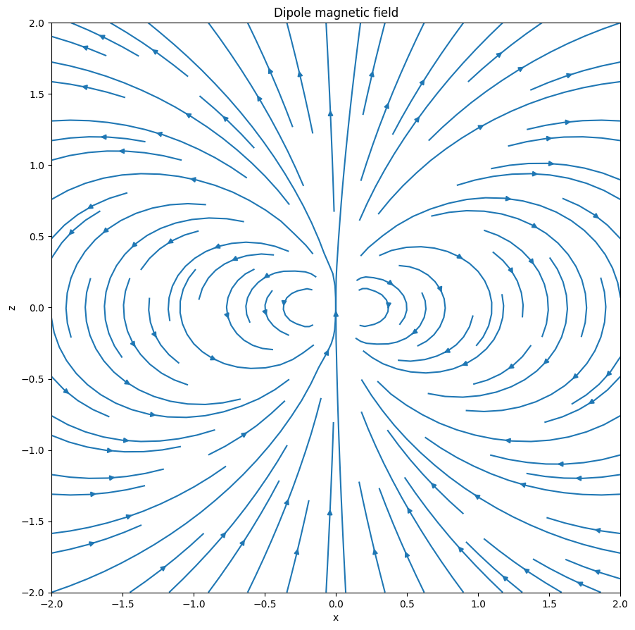
Common magnetostatic fields, like those from a magnetic dipole, can be generated and added to a plasma object.

dipole = magnetostatics.MagneticDipole(
    np.array([0, 0, 1]) * u.A * u.m * u.m, np.array([0, 0, 0]) * u.m
)
print(dipole)

MagneticDipole(moment=[0. 0. 1.]m2 A, p0=[0. 0. 0.]m)

First, we will initialize a plasma on which the magnetic field will be calculated.

plasma = Plasma3D(
    domain_x=np.linspace(-2, 2, 30) * u.m,
    domain_y=np.linspace(0, 0, 1) * u.m,
    domain_z=np.linspace(-2, 2, 20) * u.m,
)

Let’s then add the dipole field to it, and plot the results.

plasma.add_magnetostatic(dipole)

X, Z = plasma.grid[0, :, 0, :], plasma.grid[2, :, 0, :]
U = plasma.magnetic_field[0, :, 0, :].value.T  # because grid uses 'ij' indexing
W = plasma.magnetic_field[2, :, 0, :].value.T  # because grid uses 'ij' indexing

plt.figure()
plt.axis("square")
plt.xlim(-2, 2)
plt.ylim(-2, 2)
plt.xlabel("x")
plt.ylabel("z")
plt.title("Dipole magnetic field")
plt.streamplot(plasma.x.value, plasma.z.value, U, W)
plt.show()

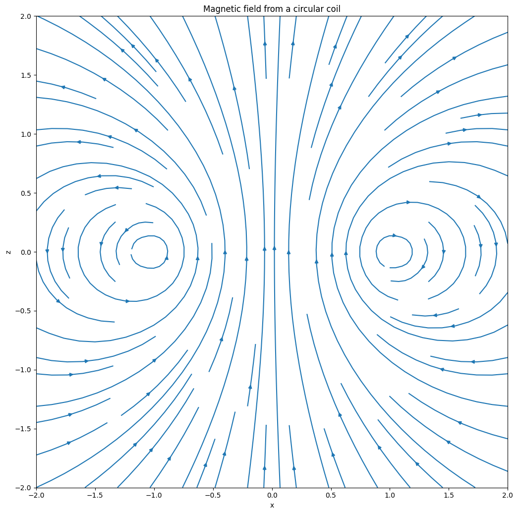
Next let’s calculate the magnetic field from a current-carrying loop with CircularWire.

cw = magnetostatics.CircularWire(
    np.array([0, 0, 1]), np.array([0, 0, 0]) * u.m, 1 * u.m, 1 * u.A
)
print(cw)

CircularWire(normal=[0. 0. 1.], center=[0. 0. 0.]m, radius=1.0m, current=1.0A)

Let’s initialize another plasma object, add the magnetic field from the circular wire to it, and plot the result.

plasma = Plasma3D(
    domain_x=np.linspace(-2, 2, 30) * u.m,
    domain_y=np.linspace(0, 0, 1) * u.m,
    domain_z=np.linspace(-2, 2, 20) * u.m,
)

plasma.add_magnetostatic(cw)

X, Z = plasma.grid[0, :, 0, :], plasma.grid[2, :, 0, :]
U = plasma.magnetic_field[0, :, 0, :].value.T  # because grid uses 'ij' indexing
W = plasma.magnetic_field[2, :, 0, :].value.T  # because grid uses 'ij' indexing

plt.figure()
plt.axis("square")
plt.xlim(-2, 2)
plt.ylim(-2, 2)
plt.xlabel("x")
plt.ylabel("z")
plt.title("Magnetic field from a circular coil")
plt.tight_layout()
plt.streamplot(plasma.x.value, plasma.z.value, U, W)
plt.show()

A circular wire can be described as parametric equation and converted to a GeneralWire. Let’s do that, and check that the resulting magnetic fields are close.

gw_cw = cw.to_GeneralWire()

print(gw_cw.magnetic_field([0, 0, 0]) - cw.magnetic_field([0, 0, 0]))

[ 0.00000000e+00  0.00000000e+00 -4.13416205e-12] T

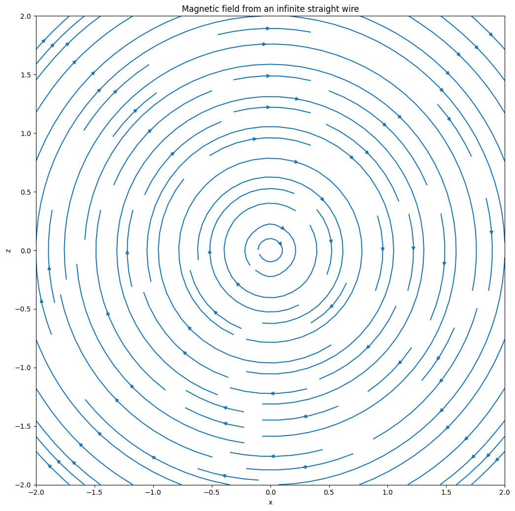
Finally, let’s use InfiniteStraightWire to calculate the magnetic field from an infinite straight wire, add it to a plasma object, and plot the results.

iw = magnetostatics.InfiniteStraightWire(
    np.array([0, 1, 0]), np.array([0, 0, 0]) * u.m, 1 * u.A
)
print(iw)

InfiniteStraightWire(direction=[0. 1. 0.], p0=[0. 0. 0.]m, current=1.0A)

plasma = Plasma3D(
    domain_x=np.linspace(-2, 2, 30) * u.m,
    domain_y=np.linspace(0, 0, 1) * u.m,
    domain_z=np.linspace(-2, 2, 20) * u.m,
)

plasma.add_magnetostatic(iw)

X, Z = plasma.grid[0, :, 0, :], plasma.grid[2, :, 0, :]
U = plasma.magnetic_field[0, :, 0, :].value.T  # because grid uses 'ij' indexing
W = plasma.magnetic_field[2, :, 0, :].value.T  # because grid uses 'ij' indexing

plt.figure()
plt.title("Magnetic field from an infinite straight wire")
plt.axis("square")
plt.xlim(-2, 2)
plt.ylim(-2, 2)
plt.xlabel("x")
plt.ylabel("z")
plt.tight_layout()
plt.streamplot(plasma.x.value, plasma.z.value, U, W)
plt.show()