This page was generated by nbsphinx from docs/notebooks/formulary/cold_plasma_tensor_elements.ipynb.
Interactive online version: .

Cold Magnetized Plasma Dielectric Permittivity Tensor

This notebook shows how to calculate the values of the cold plasma tensor elements for various electromagnetic wave frequencies.

%matplotlib inline

import astropy.units as u
import matplotlib.pyplot as plt
import numpy as np
from astropy.visualization import quantity_support

from plasmapy.formulary import (
    cold_plasma_permittivity_LRP,
    cold_plasma_permittivity_SDP,
)

For more information, check out the documentation on cold_plasma_permittivity_SDP and cold_plasma_permittivity_LRP.

Let’s use astropy.units to define some parameters, such as the magnetic field magnitude, plasma species, and densities.

B = 2 * u.T
species = ["e", "D+"]
n = [1e18 * u.m**-3, 1e18 * u.m**-3]

Let’s pick some frequencies in the radio frequency range.

f_min = 1 * u.MHz
f_max = 200 * u.GHz

f = np.geomspace(f_min, f_max, num=5000).to(u.Hz)

Next we convert these frequencies to angular frequencies. To do this we must specify an equivalency between a cycle per second and a hertz. The reasons why are described in the section of PlasmaPy’s documentation on angular frequencies.

ω_RF = f.to(u.rad / u.s, equivalencies=[(u.Hz, u.cycle / u.s)])

In a Jupyter notebook, we can type \omega and press tab to get “ω”.

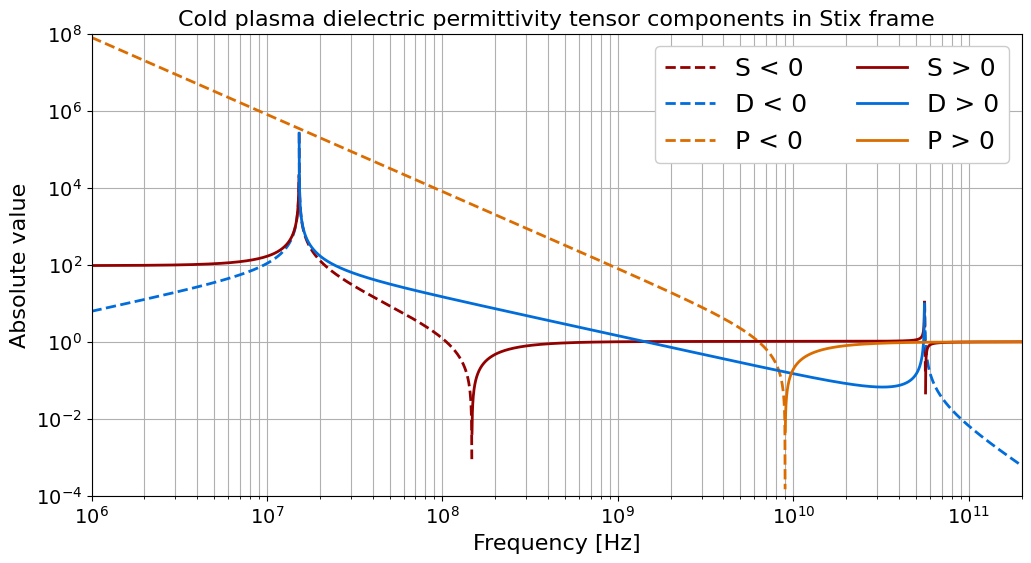
Now we are ready to calculate the \(S\) (sum), \(D\) (difference), and \(P\) (plasma) components of the dielectric tensor in the “Stix” frame with \(B ∥ ẑ\). This notation is from Stix 1992.

S, D, P = cold_plasma_permittivity_SDP(B=B, species=species, n=n, omega=ω_RF)

Next we will filter the negative and positive values so that they can be plotted separately. We’ll be doing this multiple times, so let’s create a function using the numpy.ma module for working with masked arrays.

def filter_negative_and_positive_values(arr):
    """
    Return an array with only negative values of ``arr``
    and an array with only positive values of ``arr``.
    Each element of these arrays that does not meet the
    condition are replaced with `~numpy.nan`.
    """
    arr_neg = np.ma.masked_greater_equal(arr, 0).filled(np.nan)
    arr_pos = np.ma.masked_less_equal(arr, 0).filled(np.nan)
    return arr_neg, arr_pos

Let’s apply this function to S, D, and P.

S_neg, S_pos = filter_negative_and_positive_values(S)
D_neg, D_pos = filter_negative_and_positive_values(D)
P_neg, P_pos = filter_negative_and_positive_values(P)

Because we are using Quantity objects, we will need to call quantity_support before plotting the results.

quantity_support()

<astropy.visualization.units.quantity_support.<locals>.MplQuantityConverter at 0x7fa3f34f9c40>

While we’re at it, let’s specify a few colorblind friendly colors to use in the plots.

red, blue, orange = "#920000", "#006ddb", "#db6d00"

Let’s plot the elements of the cold plasma dielectric tensor in the Stix frame.

ylim = (1e-4, 1e8)

plt.figure(figsize=(12, 6))

plt.semilogx(f, abs(S_neg), red, lw=2, ls="--", label="S < 0")
plt.semilogx(f, abs(D_neg), blue, lw=2, ls="--", label="D < 0")
plt.semilogx(f, abs(P_neg), orange, lw=2, ls="--", label="P < 0")

plt.semilogx(f, S_pos, red, lw=2, label="S > 0")
plt.semilogx(f, D_pos, blue, lw=2, label="D > 0")
plt.semilogx(f, P_pos, orange, lw=2, label="P > 0")

plt.ylim(ylim)
plt.xlim(f_min, f_max)

plt.title(
    "Cold plasma dielectric permittivity tensor components in Stix frame", size=16
)

plt.xlabel("Frequency [Hz]", size=16)
plt.ylabel("Absolute value", size=16)

plt.yscale("log")

plt.grid(True, which="major")
plt.grid(True, which="minor")

plt.tick_params(labelsize=14)

plt.legend(fontsize=18, ncol=2, framealpha=1)

plt.show()

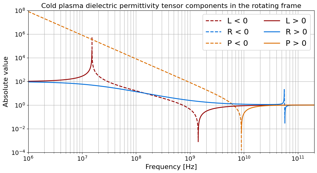
Next let’s get the dielectric permittivity tensor elements in the “rotating” basis where the tensor is diagonal and with \(B ∥ ẑ\). We will use cold_plasma_permittivity_LRP to get the left-handed circular polarization tensor element \(L\), the right-handed circular polarization tensor element \(R\), and the plasma component \(P\).

L, R, P = cold_plasma_permittivity_LRP(B, species, n, ω_RF)

Let’s use the function from earlier to prepare for plotting.

L_neg, L_pos = filter_negative_and_positive_values(L)
R_neg, R_pos = filter_negative_and_positive_values(R)
P_neg, P_pos = filter_negative_and_positive_values(P)

Now we can plot the tensor components rotating frame too.

plt.figure(figsize=(12, 6))

plt.semilogx(f, abs(L_neg), red, lw=2, ls="--", label="L < 0")
plt.semilogx(f, abs(R_neg), blue, lw=2, ls="--", label="R < 0")
plt.semilogx(f, abs(P_neg), orange, lw=2, ls="--", label="P < 0")

plt.semilogx(f, L_pos, red, lw=2, label="L > 0")
plt.semilogx(f, R_pos, blue, lw=2, label="R > 0")
plt.semilogx(f, P_pos, orange, lw=2, label="P > 0")

plt.ylim(ylim)
plt.xlim(f_min, f_max)

plt.title(
    "Cold plasma dielectric permittivity tensor components in the rotating frame",
    size=16,
)

plt.xlabel("Frequency [Hz]", size=16)
plt.ylabel("Absolute value", size=16)

plt.yscale("log")

plt.grid(True, which="major")
plt.grid(True, which="minor")

plt.tick_params(labelsize=14)

plt.legend(fontsize=18, ncol=2, framealpha=1)

plt.show()