This page was generated by nbsphinx from docs/notebooks/formulary/iter.ipynb.
Interactive online version: .

Analysing ITER parameters

Let’s try to look at ITER plasma conditions using plasmapy.formulary.

%matplotlib inline

import astropy.units as u
import matplotlib.pyplot as plt
import numpy as np

from plasmapy import formulary

The radius of electric field shielding clouds, also known as the Debye_length(), would be

electron_temperature = 8.8 * u.keV
electron_concentration = 10.1e19 / u.m**3
print(formulary.Debye_length(electron_temperature, electron_concentration))

6.939046810942984e-05 m

Note that we can also neglect the unit for the concentration, as m\(^{-3}\) is the a standard unit for this kind of Quantity:

print(formulary.Debye_length(electron_temperature, 10.1e19))

6.939046810942984e-05 m

WARNING: UnitsWarning: The argument 'n_e' to function Debye_length() has no specified units. Assuming units of 1 / m3. To silence this warning, explicitly pass in an astropy Quantity (e.g. 5. * astropy.units.cm) (see http://docs.astropy.org/en/stable/units/) [plasmapy.utils.decorators.validators]

Assuming the magnetic field as 5.3 T (which is the value at the major radius):

B = 5.3 * u.T

print(formulary.gyrofrequency(B, particle="e"))

print(formulary.gyroradius(B, T=electron_temperature, particle="e"))

932174605709.2465 rad / s

6.0740821128350554e-05 m

/home/docs/checkouts/readthedocs.org/user_builds/plasmapy/envs/latest/lib/python3.12/site-packages/plasmapy/utils/decorators/checks.py:1405: RelativityWarning: thermal_speed is yielding a velocity that is 18.559% of the speed of light. Relativistic effects may be important.
  warnings.warn(

The electron inertial_length() would be

print(formulary.inertial_length(electron_concentration, particle="e"))

0.0005287720427518426 m

In these conditions, they should reach thermal velocities of about

print(formulary.thermal_speed(T=electron_temperature, particle="e"))

55637426.422858626 m / s

/home/docs/checkouts/readthedocs.org/user_builds/plasmapy/envs/latest/lib/python3.12/site-packages/plasmapy/utils/decorators/checks.py:1405: RelativityWarning: thermal_speed is yielding a velocity that is 18.559% of the speed of light. Relativistic effects may be important.
  warnings.warn(

The Langmuir wave plasma_frequency() should be on the order of

print(formulary.plasma_frequency(electron_concentration, particle="e-"))

566959736448.652 rad / s

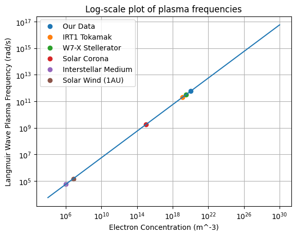
Let’s try to recreate some plots and get a feel for some of these quantities. We will also compare our data to real-world plasma situations.

n_e = np.logspace(4, 30, 100) / u.m**3
plt.plot(n_e, formulary.plasma_frequency(n_e, particle="e-"))
plt.scatter(
    electron_concentration,
    formulary.plasma_frequency(electron_concentration, particle="e-"),
    label="Our Data",
)

# IRT1 Tokamak Data
# http://article.sapub.org/pdf/10.5923.j.jnpp.20110101.03.pdf
n_e = 1.2e19 / u.m**3
T_e = 136.8323 * u.eV
B = 0.82 * u.T
plt.scatter(n_e, formulary.plasma_frequency(n_e, particle="e-"), label="IRT1 Tokamak")

# Wendelstein 7-X Stellarator Data
# https://nucleus.iaea.org/sites/fusionportal/Shared%20Documents/FEC%202016/fec2016-preprints/preprint0541.pdf
n_e = 3e19 / u.m**3
T_e = 6 * u.keV
B = 3 * u.T
plt.scatter(
    n_e, formulary.plasma_frequency(n_e, particle="e-"), label="W7-X Stellerator"
)

# Solar Corona
n_e = 1e15 / u.m**3
T_e = 1 * u.MK
B = 0.005 * u.T
T_e.to(u.eV, equivalencies=u.temperature_energy())
plt.scatter(n_e, formulary.plasma_frequency(n_e, particle="e-"), label="Solar Corona")

# Interstellar (warm neutral) Medium
n_e = 1e6 / u.m**3
T_e = 5e3 * u.K
B = 0.005 * u.T
T_e.to(u.eV, equivalencies=u.temperature_energy())
plt.scatter(
    n_e, formulary.plasma_frequency(n_e, particle="e-"), label="Interstellar Medium"
)

# Solar Wind at 1 AU
n_e = 7e6 / u.m**3
T_e = 1e5 * u.K
B = 5e-9 * u.T
T_e.to(u.eV, equivalencies=u.temperature_energy())
plt.scatter(
    n_e, formulary.plasma_frequency(n_e, particle="e-"), label="Solar Wind (1AU)"
)

plt.xlabel("Electron Concentration (m^-3)")
plt.ylabel("Langmuir Wave Plasma Frequency (rad/s)")
plt.grid()
plt.xscale("log")
plt.yscale("log")
plt.legend()
plt.title("Log-scale plot of plasma frequencies")
plt.show()