This page was generated by nbsphinx from docs/notebooks/formulary/distribution.ipynb.
Interactive online version: .

%matplotlib inline

1D Maxwellian distribution function

We import the usual modules, and the hero of this notebook, the Maxwellian 1D distribution:

import astropy.units as u
import matplotlib.pyplot as plt
import numpy as np
from astropy.constants import k_B, m_e

Take a look at the docs to Maxwellian_1D() for more information on these.

Given we’ll be plotting, import astropy’s quantity support:

from astropy.visualization import quantity_support

from plasmapy.formulary import Maxwellian_1D

quantity_support()

<astropy.visualization.units.quantity_support.<locals>.MplQuantityConverter at 0x7f9e15bef7d0>

As a first example, let’s get the probability density of finding an electron with a speed of 1 m/s if we have a plasma at a temperature of 30 000 K:

p_dens = Maxwellian_1D(
    v=1 * u.m / u.s, T=30000 * u.K, particle="e", v_drift=0 * u.m / u.s
)
print(p_dens)

5.916328704912825e-07 s / m

Note the units! Integrated over speed, this will give us a probability. Let’s test that for a bunch of particles:

T = 3e4 * u.K
dv = 10 * u.m / u.s
v = np.arange(-5e6, 5e6, 10) * u.m / u.s

Check that the integral over all speeds is 1 (the particle has to be somewhere):

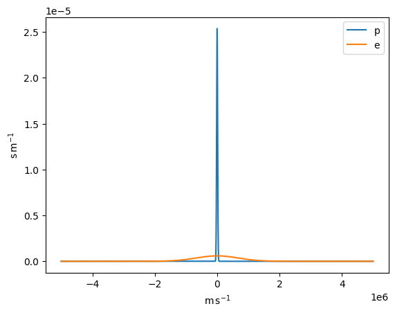
for particle in ["p", "e"]:
    pdf = Maxwellian_1D(v, T=T, particle=particle)
    integral = (pdf).sum() * dv
    print(f"Integral value for {particle}: {integral}")
    plt.plot(v, pdf, label=particle)
plt.legend()

Integral value for p: 1.0000000000000002
Integral value for e: 0.9999999999998787

<matplotlib.legend.Legend at 0x7f9e500f8bf0>

The standard deviation of this distribution should give us back the temperature:

std = np.sqrt((Maxwellian_1D(v, T=T, particle="e") * v**2 * dv).sum())
T_theo = (std**2 / k_B * m_e).to(u.K)

print("T from standard deviation:", T_theo)
print("Initial T:", T)

T from standard deviation: 29999.999999792235 K
Initial T: 30000.0 K